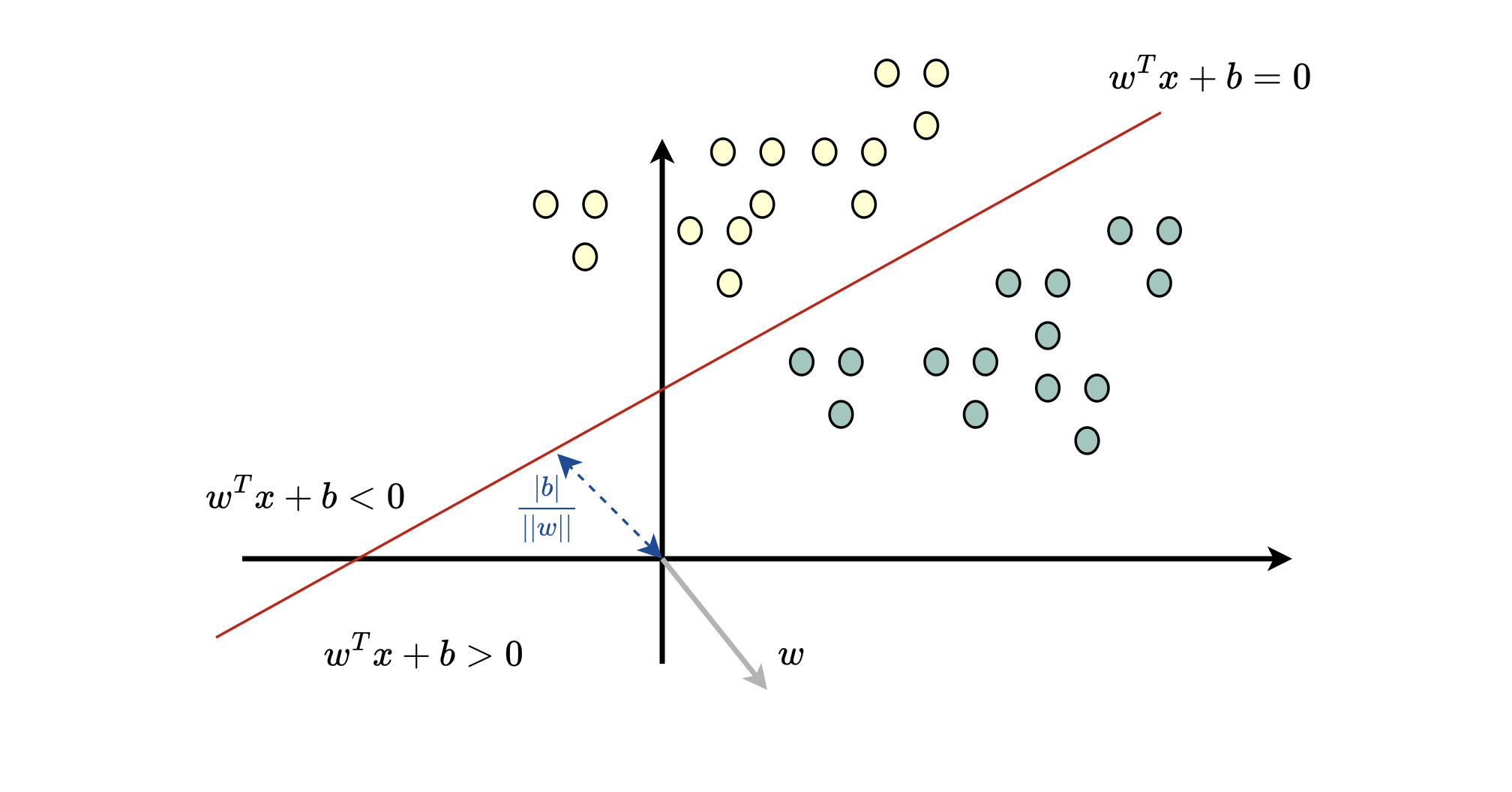
Given a dataset \( \mathbf {D} = \{(x_i, y_i)\}_{i=1}^n, x_i \in \mathbb {R}^d,\; y_i \in \{\pm 1\},\) a classifier is a function with adjustable parameters \(\theta \), \( \mathbf {f}_{\theta }: \mathbb {R}^d \rightarrow \{\pm 1\}\), that predicts the output label conditioned on \(x_i\). For example, inferring whether the behavior of a given program is malicious is a classification problem, where the label could be \(-1\) for malicious and \(1\) for benign. The goal is to have \(\mathbf {f}_{\theta }(x_i) \approx y_i\).
A linear classifier has a score of the form
Where \(\theta = \{ w,b\}\), \(b\) is the bias that shifts the decision boundary and \(w\) determines the orientation of the decision boundary (given by \(w^T x + b = 0\) ). If \(w^T x + b \geq 0\) then the predicted label is 1 otherwise -1. The classifier is then defined as
where
If a linear classifier classifies the data correctly, then the data is said to be linearly separable. More formally, a dataset is linearly separable if there exist \(w\) and \(b\), i.e., a hyperplane, such that
The minimum margin, i.e distance to closest sample, is given by:
Where we divide by \(||w||\) otherwise the projection is scaled by the size of \(w\). We multiply by \(y_i\) so that the margin is always positive for correctly classified samples, regardless of which side of the hyperplane they lie (one can also just use \(\frac {|w^T x_i + b|}{\|w\|} )\). The signed distance to the hyperplane is \(\frac {w^T x_i + b}{\|w\|}\); a negative value indicates that the sample lies on the negative side of the hyperplane. One algorithm for finding such a separating hyperplane is the Perceptron Algorithm or Gradient Ascent.
One can formulate the search for the maximum margin separating hyperplane as the following constrained optimization problem:
Given the produced score \(w^T \mathbf {x} + b\), one can turn it into a proper probability distribution using the sigmoid function:
which parameterizes the Bernoulli distribution with probability mass \(p_{\theta }(\mathbf {y} \mid \mathbf {x}) = (p_{\theta }(y = 1 \mid \mathbf {x}))^{\frac {1+y}{2}} (1-p_{\theta }(y = 1 \mid \mathbf {x}))^{\frac {1-y}{2}}\). This makes sense because \(p_{\theta }(y = 1 \mid \mathbf {x}) > \frac {1}{2}\) if and only if \(w^Tx + b> 0\).
Now, consider the scenario where we have \(L\) labels, then the classifier produces one score per class, we could write the output as \(s_{\theta }(x) = Wx + b \in \mathbb {R}^{L}\), where \(s_{\theta }(x)\) is commonly referred to as the logits. Here, the input is projected onto \(L\) different weight vectors, each with its own bias and the predicted class corresponds to the index with the highest score i.e \(\arg \max _k (Wx+b)_k\). The classifier is defined as \(\mathbf {f}_{\theta }(x) = \arg \max _{k \in \{1,...,L\}} (Wx + b)_k\). One way to learn the parameters \(W \in \mathbb {R}^{L \times d}\) and \(b \in \mathbb {R}^{L}\) is to use the Multiclass Perceptron algorithm or Gradient Ascent .
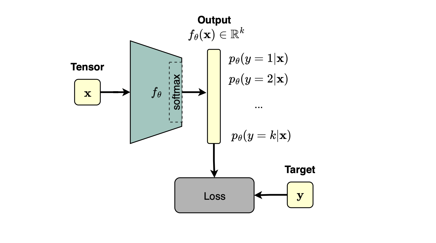
Similar to the binary case, one can turn the score function into a proper conditional distribution by using the softmax operation \( p_{\theta }(y=k \mid x) = \operatorname {softmax}(s_{\theta }(x))_k \). It makes sense because the softmax preserves ordering. The probability vector \(\pi = (\pi _1,...,\pi _L)\) where \(\pi _k:= p_{\theta }(y=k \mid x)\) and \(\sum _{k=1}^{L} \pi _k = 1\) parametrizes a categorical distribution \(\text {Cat}(y, \pi = \operatorname {softmax}(Wx+b))\) with the following probability mass function:
Now remember, we learned that we can interpret the output of a model as the parameters of a probability distribution. Later, we will see how deep neural networks are trained to learn these parameters so that the resulting conditional distribution approximates the empirical conditional distribution using maximum likelihood estimation. Parametrizing a distribution \(p(\mathbf {x})\) with neural networks provides more flexibility than, for instance, parametrizing the distribution with a linear layer. However, this increased flexibility also comes at a cost, as the resulting models can be more difficult to train, and some quantities of interest (e.g., likelihood or data density) may no longer be tractable in closed form (e.g., in a VAE), requiring us, for instance, to optimize a lower bound instead (we will discuss this later). Additionally, using neural networks to parametrize densities can introduce an identifiability problem. Basically, two learned models with different parameters or weights can produce two manifolds that are identical, and thus we can parametrize the same manifold in different ways. This is known as a reparametrization issue or an identifiability problem [1, 2, 3]. In this case, plotting and inspecting the latent space may not be a good idea for analysis. An example of an identifiable distribution is the Gaussian distribution, as changing its parameters (its mean and variance) results in a different statistical model. Probabilistic PCA [4] and densities parametrized by neural networks are generally not identifiable (e.g., a VAE).
Linear classification is often insufficient because its decision boundary is restricted to a hyperplane in the original input space. In many practical problems, the target classes are not linearly separable in this space. Several nonlinear transformations may therefore be required to map the input to a representation in which the classes become linearly separable. This is one of the motivations behind deep neural networks.
Deep learning consists of learning a sequence of transformations stacked together, where each layer receives the output of the previous layer, applies a linear transformation followed by a nonlinear activation function, and produces an output for the next layer. This is why it is called deep, as many layers are stacked together, and learning, because the parameters of these transformations, typically projection matrices for fully connected layers or kernels for convolutional layers, are learned from the dataset.
Binary Classification
In the field of machine and deep learning, we assume that the dataset \( \mathbb {D} = \{(x_i,y_i)\mid x_i\in \mathbb {X},\,y_i\in \mathbb {Y}\}, \) was generated through a random sampling process following unknown data distribution \(p_{\mathrm {data}}(x,y)\), that is, \((x_i,y_i)\sim p_{\mathrm {data}}(x,y)\). We do not get to know this distribution. However, we can approximate it using the empirical distribution.
The empirical joint distribution is given by
while the empirical marginal distribution of \(x\) is
Recall that in binary classification, the goal is to learn a mapping from the input space \(\mathbb {X}\) to the label space \(\mathbb {Y}\), \( f_\theta (x)\in \mathbb {Y} =\{0,1\} \).
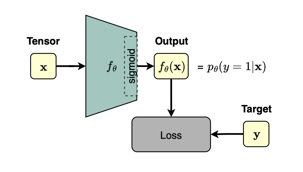
Instead of learning to map to the label directly, we will instead learn to predict, i.e interpret \(f_\theta (x)\) as \( p_\theta (y=1\mid x)\). The output of the model \(f_\theta (x)\) then parameterizes the Bernoulli distribution \(p_\theta (y\mid x)\):
or if you will
We want to find \(\theta ^{*} := \arg \min _\theta \mathbb {E}_{(x,y)\sim p_{\mathrm {\text {data}}}(x,y)} \left ( -\log p_\theta (y\mid x) \right ) = \arg \min _\theta H(p_{\text {data}}(y|x),p_{\theta }(y|x)\mathbf | p_\text {data}(x)) \)
That is, the objective function of supervised learning is to estimate the conditional (cross) entropy which measure distance between two densities. In fact, mimnimizing the cross entropy is the same as minimizing the KL divergence, which measures the discrepancy between the true conditional distribution and the model conditional distribution \(p_{\theta }(y|x)\) (as we can drop the parameter independent term), that is, \(\arg \min _\theta H(p_{\text {data}}(y|x),p_{\theta }(y|x)\mathbf | p_\text {data}(x)) = \arg \min _\theta D_{KL}(p_{data}(y|x),p_{\theta }(y|x)\mathbf | p_{\text {data}}(x) )\).
However, we do not know \(p_{\mathrm {data}}(x,y)\), so we will approximate it using the empirical distribution, that is, minimizing the negative conditional log-likelihood of the dataset \(\mathbb {D}\) (empirical cross entropy):
By the weak law of large numbers \(\mathbf {L}_{\hat {p}_{\text {data}}}(\theta )\) converges to \(\mathbb {E}_{(x,y)\sim p_{\mathrm {\text {data}}}(x,y)} \left ( -\log p_\theta (y\mid x) \right )\) and thus we can justify using the empirical negative conditional log-likelihood to estimate \(\theta ^{*}\).
Using the Bernoulli probability mass function definition,
We can define the loss (which tell us how bad the model is at prediction) as
The goal is then
where
Multiclass Classification
For multiclass classification, we parameterize a categorical distribution \(p_\theta (y\mid x)\).
The model produces a vector of scores followed by a softmax, resulting in
where \(K\) is the number of classes and
The categorical distribution can be written as
We want to find
As in the binary case, this corresponds to minimizing the conditional cross-entropy
Since
and the first term does not depend on \(\theta \), minimizing the conditional cross-entropy is equivalent to minimizing the conditional KL divergence. However, again we do not know \(p_{\mathrm {data}}(x,y)\), so we approximate it using the empirical distribution. We obtain the MLE
Using the categorical probability mass function,
For each sample, the inner term can also be written as
The loss can then be formulated as
For the empirical conditional distribution,
and therefore we can equivalently write
By the weak law of large numbers, for a fixed \(\theta \),
Deep learning models can broadly be divided into two categories: discriminative models and generative models. Discriminative models learn the conditional distribution \(p_\theta (y \mid x)\), where \(x\) denotes the input and \(y\) the corresponding target. The objective is to approximate the unknown data distribution \(p_{\text {data}}(y \mid x)\). For example, in binary classification, the output of the neural network is interpreted as the parameter of a Bernoulli distribution, as covered earlier, \(p_\theta (y=1\mid x)=f_\theta (x)\) where \(f_\theta (\cdot )\) denotes the deep neural network. Given training samples \(\{(x_i,y_i)\}\) assumed to be sampled from the unknown distribution \(p_{\text {data}}(x,y)\), the model is typically trained by minimizing the cross-entropy loss, which is equivalent to maximizing the likelihood of the observed labels or, equivalently, minimizing the KL divergence between the true conditional distribution \(p_{\text {data}}(y\mid x)\) and the model distribution \(p_\theta (y\mid x)\). The empirical cross-entropy converges in probability to the conditional cross-entropy as the number of samples increases (\(n\rightarrow +\infty \)).
Generative models, on the other hand, learn how the data itself is generated by approximating the data distribution \( p_{\text {data}}(x) \). For example, Generative Adversarial Networks or GANs learn an implicit distribution by mapping samples drawn from a simple prior distribution \(p(z)\), typically a standard Gaussian, through a generator network \(G_\theta (z)\). On the other hand, Variational Autoencoders or VAEs explicitly introduce a latent variable \(z\) and model the joint distribution \( p_\theta (x,z)=p_\theta (x\mid z)p(z)\), where \(p(z)\) is a predefined prior, usually a standard Gaussian. The data likelihood is then given by \( p_\theta (x) = \int p_\theta (x\mid z)p(z)\,dz, \) which is generally intractable to compute exactly. Large Language Models or LLMs are also generative models. They learn the joint probability distribution of a sequence of tokens by factorizing it using the chain rule (autoregressive or AR modeling), \( p_{\theta }(x_1,\ldots ,x_n) = p_{\theta }(x_1) \prod _{i=2}^{n} p_{\theta }(x_i\mid x_1,\ldots ,x_{i-1}). \). Training consists of learning each conditional distribution so that the model can accurately predict the next token given all previous ones (which is easier than generating celebrity faces). Once trained, the model can either compute the likelihood of a sequence or generate new text by repeatedly sampling or selecting the next token from the learned conditional distribution.
In the field of deep learning, we assume that the data was generated from some unknown distribution (i.e there is a data-generating process behind), and we attempt to approximate it using a parametric model \(p_\theta (x)\). We observe random samples \(\{x_i\}_{i=1}^n\) where \(x_i \sim p_{\text {data}}(x)\) (the datapoints are assumed to be iid). The goal of learning is to find \(\theta \) such that \(p_\theta (x) \approx p_{\text {data}}(x)\) i.e., we approximate the underlying data distribution (using the empirical distribution). Once we have learned \(p_\theta (x)\), we can generate artificial or synthetic samples. However, under the manifold hypothesis, \(p_{\text {data}}(x)\) is concentrated on a low-dimensional manifold embedded in a very high-dimensional ambient space. This motivates introducing a lower-dimensional latent space from which the observed data can be generated.
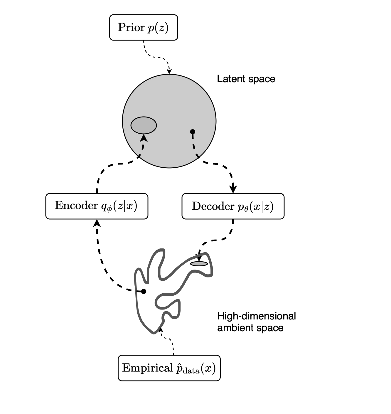
We learn how to transform a simple fixed distribution in latent space, for example \(p(z)=\text {Normal}(0,I)\), into the data distribution. Rather than learning a mapping as in GANs, we use conditional modeling and learn the conditional density \(p_\theta (x \mid z)\). More precisely, we model
To estimate \(p_{\text {data}}(x \mid z)\), we use a deep neural network whose output parameterizes the conditional distribution \(p_\theta (x \mid z)\) (i.e., the decoder parameterizes this distribution). We assume that the observed data were generated from latent variables, i.e., pairs \((x,z)\) were generated, but only \(x\) is observed while \(z\) remains hidden.
Since \(x\) and \(z\) are dependent, we can write the marginal likelihood as (assuming the prior is fixed and known)
Our objective is to learn \(\theta \) such that
Unfortunately, \(p_\theta (x)\) intractable (i.e no analytic solution) because \(p_\theta (x\mid z) = \mathcal {N}\!\left (x;f_\theta (z),\sigma ^2 I\right )\) is parameterised using a multi-layer neural-network decoder, making the integral impossible to evaluate analytically. We could use naive Monte Carlo estimation by sampling a large number of latent variables from the prior \(z_k \sim p(z)\) and compute \(p_\theta (x)\) approximately
Giving
While writing the marginal likelihood as an expected value with respect to the prior distribution seems to solve the problem, it leads to an unstable estimator, as most of the sampled \(z\) values will result in likelihood values close to zero. We are likely to miss, by chance, those samples that would result in high likelihood values, thereby increasing the variance of the estimator (very large random samples are needed) [5, 6]. To see why, imagine drawing latent vectors from the prior. For a given observation \(x\), only a small subset of latent variables \(z\) are likely to explain it well. Consequently,\( p_\theta (x\mid z)\approx 0\) for most sampled \(z\). By Bayes’ rule,
this implies that the posterior places almost all of its probability mass on a very small region of the latent space, while assigning nearly zero probability to the rest.
The key idea behind Variational Autoencoder or VAE is therefore to introduce an approximate posterior distribution \(q_\phi (z\mid x)\) to produce latent variables that are likely to assign a high probability to the observation through \(p_\theta (x\mid z)\). This provides an efficient way to identify the regions of latent space that explain the data and serves as the first step toward learning a latent representation that can later be used for generation by sampling from the prior.
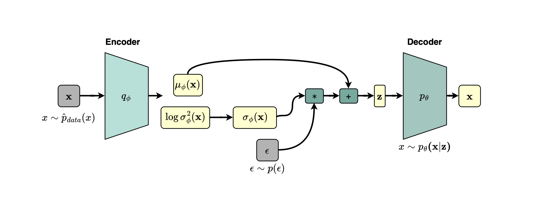
We start from the marginal likelihood
and therefore
Introducing an arbitrary distribution \(q(z)\), we can write
or,
Taking the expectation with respect to \(q(z)\),
Since \(\log p_\theta (x)\) does not depend on \(z\),
Using
we obtain
Expanding the first term gives
Since
we obtain
Therefore,
because
The term
is known as the Evidence Lower Bound or ELBO for short.
We now set
where \(q_\phi (z\mid x)\) is parameterized by an encoder with parameters \(\phi \).
The VAE objective becomes
For the empirical data distribution,
where the expectation over \(q_\phi (z\mid x_i)\) can be approximated using Monte Carlo sampling.
We assume that \(q_\phi (z\mid x)\) parameterizes a Gaussian distribution.
For a latent space of dimension \(b\),
Equivalently,
The encoder therefore outputs
or, in practice, typically
Assume the prior is
Then the KL divergence has a closed-form expression:
Therefore,
Hence, the loss can be simplified to
Now we need to to compute \( \frac {\partial \mathbf {L}}{\partial \theta } \qquad \text {and}\qquad \frac {\partial \mathbf {L}}{\partial \phi }\). Computing the gradient with respect to \(\theta \) is simple because we can use Monte Carlo sampling to eliminate expectation \(\mathbb {E}_{q_\phi (z\mid x_i)}\).
For example,
But what about \( \frac {\partial \mathbf {L}}{\partial \phi }\)
This is a little problematic because the distribution from which we sample depends on \(\phi \).
In general,
For the second term,
the closed-form expression depends explicitly on \(\phi \), and its gradient can be obtained using automatic differentiation.
The remaining problem is therefore how to compute
Instead, we use the reparameterization trick.
We write
We can therefore write
Then
The randomness has now moved from \(z\) to \(\epsilon \), whose distribution \( p(\epsilon )=\mathcal {N}(0,I)\) does not depend on \(\phi \). Consequently,
Since \(p(\epsilon )\) does not depend on \(\phi \), we can move the derivative inside the expectation:
We can now use Monte Carlo sampling. Observe that \(p_\theta (x\mid z)\) depends on \(\phi \) through \( z = \mu _\phi (x) + \sigma _\phi (x)\odot \epsilon \). For example, if the decoder distribution \(p_\theta (x\mid z)\) is Gaussian, the reconstruction term can correspond to an \(L_2\) loss.
We can therefore write the VAE objective as
Using a single Monte Carlo sample
we obtain
and the objective becomes
This objective is then trained using SGD.
GANs, or Generative Adversarial Networks (and many other generative and machine learning models like diffusion models or autoencoders) are motivated by the manifold hypothesis concept, which states that the data of interest (e.g natural images or celebrity faces) form a thin d-dimensional submanifold \(\mathbb {M}\) embedded in a high-dimensional ambient space \(\mathbb {X}\) (e.g \(\mathbb {R}^D\), where \(d<D\); d is known as intrinsic dimension while \(D\) is the ambient dimension).
GAN tries to learn a mapping from a given latent space \(\mathbb {Z}\) to \(\mathbb {M}\) and then samples from \(\mathbb {M}\) by sampling from \(\mathbb {Z}\).
In GAN, there is no explicit likelihood maximization as in a VAE (i.e it is not a likelihood-based model). Instead, there is a generator \(g_\theta (z)\) that generates a candidate sample \(x_{\text {fake}} = g_\theta (z)\), where \(g_\theta \) is a deep neural network.
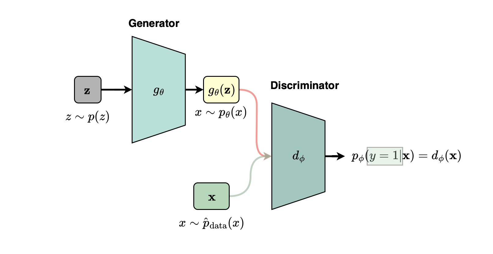
The generator is trained to fool a discriminator (binary classifier) \(d_\phi \) in an adversarial fashion. The discriminator, represented by \(d_\phi \), outputs the probability that a sample is real. The goal of the discriminator is to maximize \(\log d_\phi (x)\) for real samples \(x \sim p_{\text {data}}\), and to maximize \(\log \left (1-d_\phi (g_\theta (z))\right )\) for fake samples \(z \sim p(z)\).
The loss is the standard binary cross-entropy loss (i.e., similar to training a binary classifier) and is given by (which is equivalent to minimizing the Jensen-Shannon divergence)
As usual, we do not have access to the true data distribution, and thus we approximate it using the empirical distribution:
The term \(\mathbb {E}_{z\sim p(z)}\) is approximated using Monte Carlo sampling. During SGD training, when training the discriminator, the generator parameters are kept fixed, i.e., the generator does not learn. Similarly, when training the generator, the discriminator parameters are kept fixed. With PyTorch, this alternating training procedure is straightforward to implement.
Getting a GAN to work can be difficult due to vanishing gradients, non-convergence, instability of the adversarial equilibrium, and especially mode collapse. Mode collapse can happen when the generator learns a distribution concentrated on only a few modes or examples instead of approximating the full data distribution.
Autoregressive models are generative models that attempt to learn the underlying data distribution \(p_{\mathrm {data}}(x)\) from which the observed data are assumed to have been generated. The data is usually sequential, such as text represented as tokens; in this scenario, the model is trained to learn the token distribution. Because text is viewed as a sequence of tokens belonging to a vocabulary, the model learns the distribution that governs the world language space. The joint distribution is given by:
where \(x_{<k}=(x_1,\ldots ,x_{k-1})\). Thus, instead of directly learning \(p_\theta (x)\), we learn the conditional distributions; this is why LLMs are said to model the conditional distribution of the next token. Each conditional distribution \(p_\theta (x_k \mid x_{<k})\) is parameterized by the underlying language model with parameters \(\theta \), typically using the final-layer contextual representation at position \(k-1\) to predict the distribution over \(x_k\), that is:
where \(h_{t-1}^{(L)}\) is the final-layer contextual representation at position \(t-1\).
To make the estimation problem amenable and parameter-efficient, large language models use the same model parameters \(\theta \) to estimate all these conditional distributions. The model is trained using maximum likelihood estimation by maximizing the likelihood of the observed data, or equivalently by minimizing the negative log-likelihood. This is equivalent, up to a constant independent of \(\theta \), to minimizing \(D_{\mathrm {KL}}\left (p_{\mathrm {data}}(x)\,\|\,p_\theta (x)\right )\).
The log-likelihood objective subject to maximization is given by:
Instead of solving a maximization problem, one can minimize the negative log-likelihood (next-token prediction loss):
The expectation is approximated using Monte Carlo with samples from the training corpus, that is, the objective or loss becomes:
Where \(\mathbb {B}\) is a randomly picked batch.
Once the conditional distributions \(p_\theta (x_k\mid x_{<k})\) have been learned, their product defines \(p_\theta (x)\). The model can also be used to predict and sample the next token given a context. The sampled token is appended to the context, and this process is recursively repeated until a stopping condition is reached (e.g maximum length or end of sentence token). This is how an autoregressive LLM basically generates text.
Modern language models typically use Transformer architectures to parametrize these conditional distributions. Each \(p_\theta (x_k\mid x_{<k})\) is a categorical distribution over the vocabulary (i.e which tokens are more likely to be picked next). The Transformer produces a final-layer contextualized representation at position \(k-1\):
which has attended to the previous tokens and therefore encodes the preceding context. The network then produces one logit for each possible token by projecting this contextualized representation onto the vocabulary, and a softmax transforms these logits into probabilities:
We will delve into the details of the Transformer architecture later.
By learning each conditional distribution \(p_\theta (x_k\mid x_{<k})\), the model learns to predict the next token given a context \(x_{<k}\). During generation, a token is produced, appended to the context, and the model is invoked again until either an end-of-sentence (EOS) token is produced or predefined maximum length reached. This process is called autoregressive generation.
During training, teacher forcing is used to enable parallel computation, that is, compute the conditional probabilities ahead of time as next tokens are known (cf tranformer section). During inference, however, generation is sequential and the auto regressive property must be obeyed conservatively because the next tokens are not known.
When using LLM APIs, you will probably come across the notion of temperature; it is basically a way to drive and control the generation process, e.g., from more greedy/deterministic generation to more diverse generation (in other words it control the softness of the distribution). Let \(\boldsymbol {z}_\theta (x_{<k})\) denote the logit vector produced by the model for the token position at \(k\) (as explained earlier), \(\boldsymbol {z}_\theta (x_{<k}) \in \mathbb {R}^{|V|}\), e.g., the Transformer output where the token has the chance to look at preceding token representations. Temperature modifies the sampling distribution according to:
where \(\tau >0\) is the temperature scaling factor. For \(\tau =1\), we obtain the original token model distribution. For \(0<\tau <1\), the distribution becomes sharper, so high-probability tokens are favored more strongly and low-probability tokens are sampled less often, as the differences between the logits are amplified. As \(\tau \rightarrow 0^+\), the distribution concentrates on the token with the largest logit, converging towards greedy decoding. For \(\tau >1\), the distribution becomes flatter, and as \(\tau \rightarrow +\infty \), it tends toward a uniform distribution. Setting \(\tau =0\) is typically interpreted as greedy decoding, that is, the token with the largest logit is selected; it effectively gets a probability of \(1\), while all others get \(0\).
Given an alphabet \(\Sigma \), that is, a finite set of symbols, let \(\Sigma ^*\) denote the set of all possible finite sequences or strings over the alphabet. A vocabulary \(V\) is a finite set of strings on a given alphabet \(\Sigma \), that is, \(V \subset \Sigma *\).
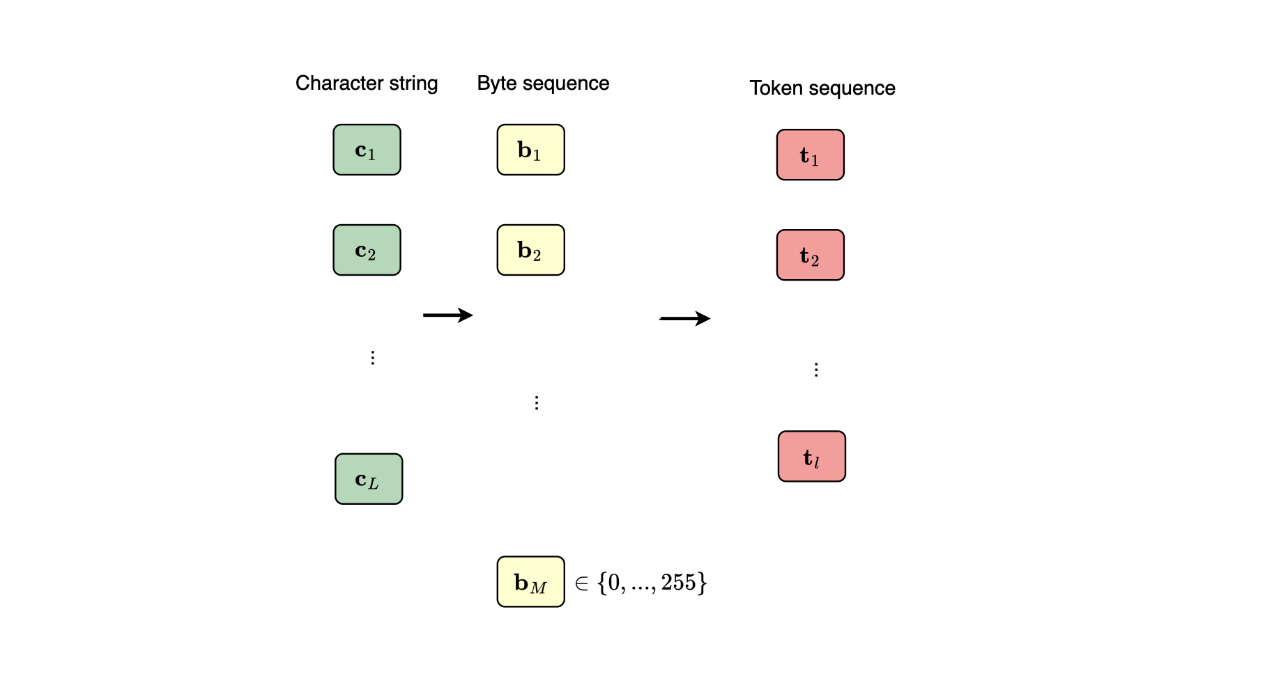
A tokenizer, denoted by \(\boldsymbol {\tau }\), breaks down a text into a sequence of tokens belonging to a target vocabulary \(V\). Formally,
where \(\Sigma \) denotes the alphabet of characters or bytes \(\{0,\ldots ,255\}\) (if we consider UTF-8 encoding), and \(V\) determines the set of all possible tokens, that is, the vocabulary which may contain words, subwords, individual characters and punctuation symbols ; which is different from usual linguistic vocabulary. In LLMs, the target vocabulary is typically learned from a training corpus.
Given a text, the tokenizer maps it to a sequence of tokens:
Next, each of these tokens can be mapped to an index using a deterministic indexing function
Each token ID is then used to index an embedding table, called the token embedding table, which provides a vector representation of the token (which we will discuss in more detail later).
Thus, a tokenizer block takes a string over an alphabet and maps it to a sequence of token indices, whose length \(\ell \) is the tokenized sequence length. If this sequence is used as the model’s input, \(\ell \) is its input context length. Each token is then embedded into a dense vector in a \(d\)-dimensional Euclidean space. Let
denote the embedding lookup. Then, for
the corresponding token embedding matrix can be written as
Thus, the text is mapped to \(\mathbb {R}^{d\times \ell }\), where each column is the vector representation of one of the \(\ell \) tokens. Here, \(\ell \) is the input sequence length, and \(\boldsymbol {X}\in \mathbb {R}^{d\times \ell }\) is the token embedding matrix that is fed into the machine learning model or LLM. Examples of tokenization algorithms include WordPiece, Unigram Language Model (UnigramLM), and Byte Pair Encoding (BPE).
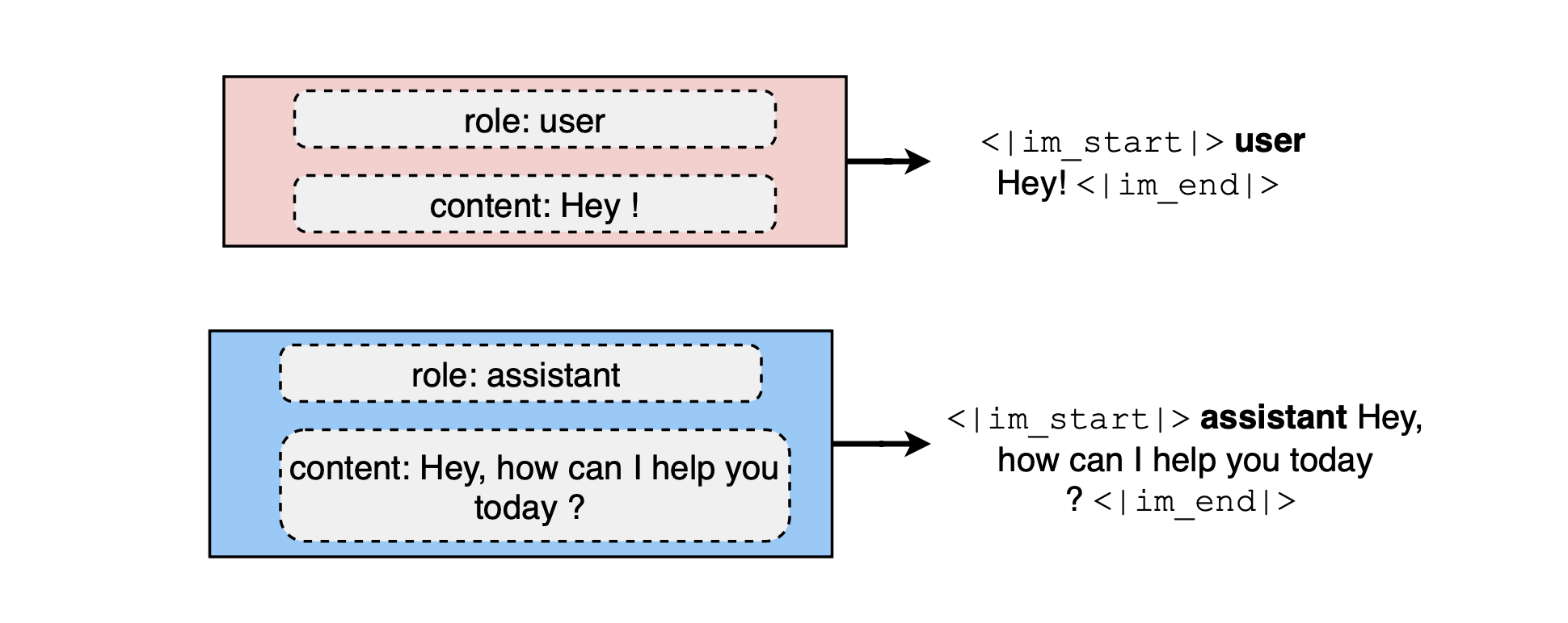
Some special tokens are also part of the tokenizer’s vocabulary, including
<|im_start|>{{role}}
{{content}}<|im_end|>
That is, the mapping from raw data
[
  {'role': 'system', 'content': 'You are a helpful security analyst'},
  {'role': 'user', 'content': 'analyze security event...'},
  {'role': 'assistant', 'content': 'Sure, here is...'}
]
could be
<|im_start|><|system|>
You are a helpful security analyst.<|im_end|>
<|im_start|><|user|>
analyze security event...<|im_end|>
<|im_start|><|assistant|>
Sure, here is...<|im_end|>
Of course, each LLM may have its own chat template. Usually, you do not need to care about the conversation formatting if you use LLM provider APIs or SDKs rather than an open-source model; you just send the conversation. This is, by the way, how you can build LLM-based agents, as covered later.
Large language models are also post-trained on tool usage or function calling, where a list of tool descriptions is presented and the model, based on the task encoded in the instruction and the payload, suggests one or more tool calls. The emitted tool calls can follow a certain schema dictated in the prompt, or special tokens can also be introduced for that purpose. For instance, Qwen (https://qwen.readthedocs.io/en/latest/getting_started/concepts.html) uses XML tags and does not introduce special tool-call tokens. Here is what the template looks like (once the chat template is applied, the tokenizer then comes into play to produce the token sequence, as explained earlier):
<|im_start|>system
# Tools
You may call one or more functions to assist with the user query.
You are provided with function signatures within <tools>tools> XML tags:
<tools>
{{JSON Schema of function 1}}
{{JSON Schema of function 2}}
tools>
For each function call, return a JSON object with function name and arguments
within <tool_call>tool_call> XML tags:
<tool_call>
{"name": <function-name>, "arguments": <args-json-object>}
tool_call>
<|im_end|>
<|im_start|>user
{{user content}}
<|im_end|>
<|im_start|>assistant
<tool_call>
{{tool call 1}}
tool_call>
<tool_call>
{{tool call 2}}
tool_call>
<|im_end|>
<|im_start|>user
<tool_response>
{{tool result 1}}
tool_response>
<tool_response>
{{tool result 2}}
tool_response>
<|im_end|>
<|im_start|>assistant
{{assistant content}}
<|im_end|>
On the other hand, Gemma 4 uses special tool tokens rather than XML tags (https://ai.google.dev/gemma/docs/core/prompt-formatting-gemma4); it uses six special tokens to manage the tool-use lifecycle.
A model naturally cannot actually call the tool itself (it samples next probable token or response). Instead, it requests a tool call, and it is the responsibility of the surrounding system to handle the call and append the tool call and its result to the chat history (harness is often used to refer to how tools and other resources like skills or components like neural memory module are organized or orchestrated and connected to the foundation model).
Additionally, especially when developing agents, large language models can use a thinking mode
in which the model emits structured reasoning (
<|im_start|>user
{{user content}}
<|im_end|>

<|im_start|>assistant
<think>
{{thinking content}}
think>

{{assistant content}}
<|im_end|>
On the other hand, Gemma 4 introduces the <|think|> special token to activate thinking and delimits internal reasoning content using special delimiters or tokens:
<|turn>system
<|think|>You are a helpful assistant.
<|tool>declaration:get_current_temperature{...}<tool|>
<turn|>

<|turn>user
What's the temperature in London?
<turn|>

<|turn>model
<|channel>thought
...
<channel|>
<|tool_call>call:get_current_temperature{
    location:<|"|>London<|"|>
}<tool_call|>
<|tool_response>
As stated earlier, the chain-of-thought can be enclosed between special tags or tokens, such as
That is, the model first autoregressively generates the reasoning tokens conditioned on the input context and then generates the final response conditioned on both the input context and the generated reasoning.
The limitation of recurrent neural networks was that inputs might be correlated and distant, resulting in the loss of critical context for accurate predictions. LSTM addressed this issue by utilizing memory cells scattered throughout the network to provide additional contextual information. However, even with LSTM, there were still limitations as you had to put your trust in the model. Additionally, encoding the complete semantics of an entire sentence into the hidden state of the last moment of the encoder in vanilla se2seq presents a significant challenge.
To overcome these limitations, the attention mechanism was introduced. The idea behind the attention mechanism is to allow the model to learn how to selectively focus on the information necessary for predicting outputs. It aims to leverage all the information from the past combining different layers with weighted averages. The attention scores are typically learned via a deep neural network.
Given query, key, and value vectors
we can arrange them column-wise as
where
We assume that the query vector \(q\) and key vector \(k\) have undergone a transformation, e.g., through a deep neural network, such that \(q^\top k\) provides a similarity score between \(q\) and \(k\).
For a query \(q_i\), we can define its output \(y_i\) as a weighted average of the value vectors using the similarity scores:
If we want to normalize the weights so that they are positive and sum to one, we apply the softmax function:
Hence,
Since
we can write
If we stack the outputs column-wise,
then
where the softmax is applied row-wise.
In scaled dot-product attention (to cope with situations where the dot product is large), we instead use
If we instead use the row-vector convention, the same expression is usually written as
Using the column-vector convention, define the similarity score as
The normalized attention weight is therefore
with
The coefficient \(\alpha _{ij}\) can be interpreted as
or \(p(k_j\mid q_i)\); given a query \(q_i\), it indicates how much attention mass should be granted to position or key \(j\). This is why LLMs are said to learn an attention distribution.
We can therefore write
Multi-head attention is an extension of attention in which multiple heads are introduced. Each head can focus on a different aspect of the sequence. Concretely, \(Q\), \(K\), and \(V\) are projected onto different subspaces, allowing the model to learn multiple kinds of relationships in parallel.
Let \(h\) denote the number of attention heads. For head \(i\), define
where, for a head dimension \(d_h\),
Each head is then
Equivalently,
The outputs of the heads are concatenated:
Finally,
where
so that
In self-attention, given
we compute the queries, keys, and values as projections of the same input:
More generally, if the query/key dimension is \(d_k\) and the value dimension is \(d_v\),
and therefore
We then compute scaled dot-product attention:
The scaling is used to prevent the dot products from becoming too large as \(d_k\) increases.
Finally,
For the multi-head version, for
we define
where
Then
and
Since we are interested in autoregressive modeling, we want to enforce the autoregressive property so that a token at position \(i\) cannot attend to future positions \(j>i\).
We introduce a causal mask
defined by
For each head, we then compute
Thus, whenever \(j>i\),
and consequently
After applying the softmax gives 0 (\(e^{-\infty }=0\)), thus attention to future positions is switched off.
The corresponding head output is
Additionally, we can add a residual connection to form the final contextual embeddings:
Finally, we can add a feed-forward neural network and normalization layer:
where the residual connection with \(X\) is already included in \(\operatorname {MaskedMultiHead}(X)\).
The final output is
The Transformer architecture has become the go-to deep learning model for various tasks. It consists of an encoder and a decoder. The encoder consists of multi-head attention layers and position-wise feed-forward sublayers. In order to compensate for the absence of a cyclic structure inherent in recurrent neural networks, which naturally capture positional information and ordering, Transformers employ positional encodings. The idea is to augment the input embedding with a fixed sinusoidal positional encoding (one can also use learned positional embeddings).
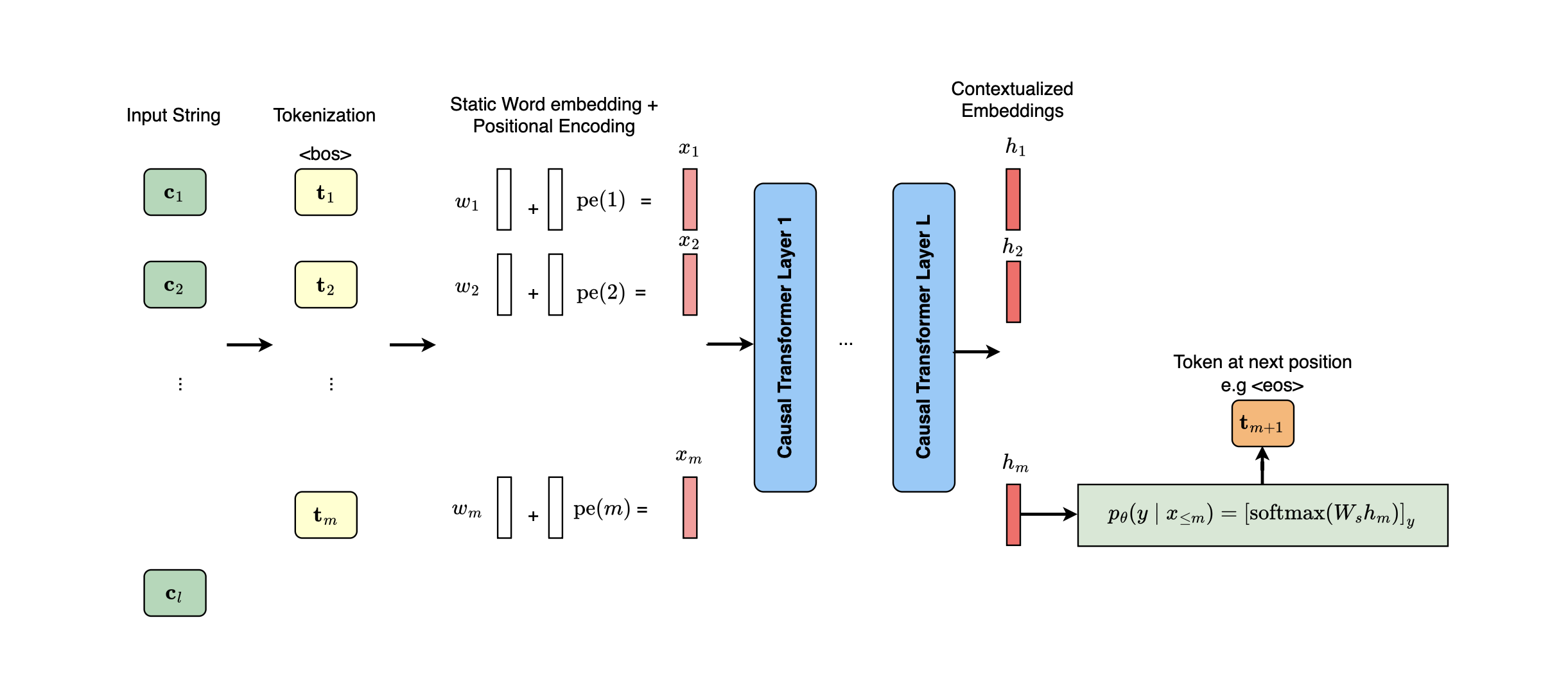
For position \(i\), the positional encoding is defined by
and
where \(j\) denotes the dimension index in the embedding space and \(d\) is the dimension of the embedding space.
For a token \(w_i\) with embedding
we define the position-aware embedding as
where
is the embedding matrix learned using backpropagation, where each column is the embedding vector associated with a token in the vocabulary \(\mathbb {V}\), and \(E_{w_i}\) denotes the column of \(E\) corresponding to the token index \(w_i\).
If
denotes the one-hot representation of the token index \(w_i\), then
For an input sequence of \(n\) tokens, define
The corresponding token-embedding matrix is therefore
where
Thus, the gradient with respect to the embedding matrix \(E\) can be written as
where
and consequently
Instead of explicitly constructing the entire sparse one-hot matrix \(O_h\), observe that
and thus the forward pass can simply select the corresponding columns of \(E\). Similarly, during the backward pass, gradients only need to be accumulated into the columns that were selected during the forward pass, with the gradients summed when the same column is selected multiple times (we will discuss the torch embedding layer later).
In matrix form, if
and
then
Transformers can be stacked, forming \(N\) layers. The encoder can be written as
followed by
The final contextual embeddings at the output of the last encoder layer are
The decoder block acts as an autoregressive language model. Its initial representation is
where
contains the positional embeddings and
contains the output embeddings generated so far, or can also be set to the ground-truth target sequence during training using teacher forcing. The first sublayer is masked multi-head self-attention:
We then use attention over the encoder representations, allowing the decoder to incorporate information from the input sequence and its own previous output:
Finally, the feed-forward sublayer gives
The position-wise feed-forward network is given by
The layer normalization operation is defined as
The final contextual embedding is therefore
This representation can be fed to a classification layer to obtain the next-token predictions. In token prediction, we use
where
At each position \(i-1\), the final contextual representation \(h_{d,i-1}^{(N)}\), which encodes the preceding context \(w_{<i}=(w_1,\ldots ,w_{i-1})\), is used to predict the next token \(w_i\):
The predicted token ID is obtained as the index of the largest logit, i.e.,
The decoder is trained to generate the sentence shifted by one position, effectively learning how to predict the next token. This is the autoregressive decoder used, for example, in GPT-type models.
At position \(t-1\), the final hidden state \(h_{t-1}\), which represents the preceding context \(x_{<t}=(x_1,\ldots ,x_{t-1})\), is projected to one logit per vocabulary token:
Then,
This parametrizes the categorical distribution over the vocabulary for the next token \(x_t\). Therefore, for a particular vocabulary token \(y\),
For an autoregressive language model, the probability of a sequence \(x=(x_1,\ldots ,x_T)\) is factorized using the chain rule as
The model is pretrained by maximizing the log-likelihood of the training sequences, or equivalently by minimizing the negative log-likelihood (the cross-entropy loss):
Using the autoregressive factorization, this becomes
And, since \(p_\theta (x_t\mid x_{<t})\) corresponds to the softmax entry associated with the ground-truth token \(x_t\),
where \(h_0\) is the hidden representation corresponding to a special beginning of sequence token \( x_{<1} = <\texttt {bos}>\).
An input string is tokenized, typically after applying a chat template, and then a set of keys and values is created by projecting the input representations using \(W_K\) and \(W_V\). The new representations for each token are then obtained. If multi-head attention is used, this operation is performed for each head and also at each layer.
During inference, one needs to obey the autoregressive property, and thus each new token is produced and then appended to the current context to form the input for the next decoding step, and so on. However, because we are obeying the autoregressive property, the keys and values of previous tokens, obtained through many GEMMs during prefill (and thus compute bound), will not change due to future tokens. Thus, recomputing them (or redoing the prefill) is unnecessary, and the keys and values for each head and each layer can be cached (and queries discarded). We call the collection of cached key and value vectors the KV cache. There are many scenarios that present opportunities for prefix caching, including agentic workloads, where the system prompt, along with tool descriptions and examples, remains the same, or when a new round consists of previously generated trajectories.
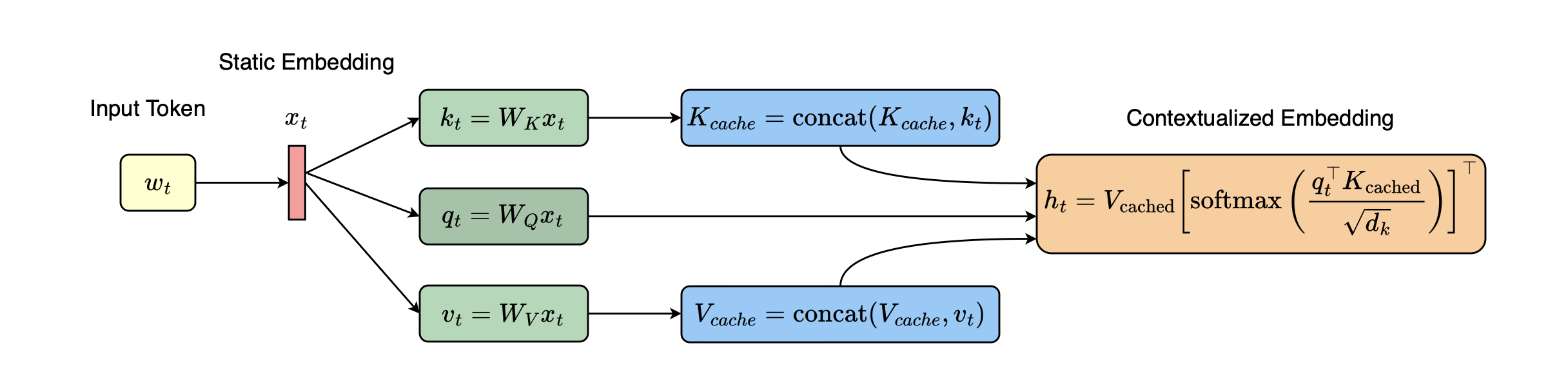
Basically, for each newly produced token now in step \(t\), we need to compute its new key and value. For example, suppose that, at a given layer and head, the cache contains
Given the dense representation \(\mathbf {x_t}\) of the new token at the input of this layer, we compute
The cache is then extended as (we append to keys and values tensors)
We do not need to recompute or cache the queries of the previous tokens, because we only need the current query \(q_t\) to attend to their cached keys and values to predict the next token. This is why we have a KV cache rather than a QKV cache. The attention output for the current token is computed as
under the column-vector convention.
Once the new hidden representation for the current token is produced by the first layer, \(h_t^{(1)}\), we continue in the same manner through all the Transformer layers:
At the final layer, the next-token distribution is obtained by applying the language-model head followed by a softmax:
We can now see that there are many matrix-vector operations involved during autoregressive decoding. Since only one token is processed at each decoding step, these operations have relatively low arithmetic intensity compared with the prefill phase. Consequently, autoregressive decoding is typically memory-bound.
A typical implementation of KV caching with prefix caching,(e.g vLLM). The basic idea is to choose a fixed block size for cache lookup. A hash is computed for the first block and checked against the cache. If it is found, the corresponding cached KV block can be reused. For the next block, the hash of the previous block is combined with the tokens of the current block to compute a new hash, which is again checked against the cache. The lookup continues until a block misses. In this case, the cached KV blocks before the miss can be reused, while the tokens starting from the first missing block must be processed through the Transformer layers to compute their KV states. A cache salt can also be used to ensure that only requests with the same salt can reuse cached KV blocks. PagedAttention was introduced to solve memory fragmentation in the KV cache by allowing blocks to be allocated as needed. FlashAttention significantly improve the efficiency of the attention computation using tiling, thereby reducing memory accesses to Keys and Values and avoiding materializing the large attention score matrix.
Knowledge distillation is a model compression technique that consists of transferring knowledge from a large teacher model to a smaller student model by mimicking the teacher’s categorical distribution; this is because the categorical distribution reveals valuable knowledge concerning other classes rather than just the hard labels. Let \(q(y=i\mid x)\) denote the teacher’s probability distribution and \(p_\theta (y=i\mid x)\) the student’s probability distribution. A common knowledge-distillation objective is the cross-entropy from the teacher distribution to the student distribution:
which is equivalent to minimizing the KL divergence, since the first term does not depend on \(\theta \):
The student probabilities are obtained from its logits through a softmax (both the teacher’s and student’s logits can be scaled by a temperature parameter). The distillation objective is typically combined with the supervised target loss (e.g., cross-entropy):
In language modeling or LLMs, the global loss is given by
where the second loss term is a KL-divergence penalty. Since the teacher distribution \(q\) does not depend on \(\theta \), this term can be written, up to a constant independent of \(\theta \), as a cross-entropy. Therefore, the loss can equivalently be written as
If we look at the source code for knowledge distillation (PyTorch Knowledge Distillation Tutorial), the implementation (using full KL divergence) is relatively simple in PyTorch. The teacher forward pass is performed inside torch.no_grad() so that no computation graph is constructed for the teacher, since its parameters are fixed. The student forward pass is performed normally, and the distillation loss is computed directly from the teacher and student logits.
def train_knowledge_distillation(
    teacher,
    student,
    train_loader,
    epochs,
    learning_rate,
    T,
    soft_target_loss_weight,
    ce_loss_weight,
    device
):

    ce_loss = nn.CrossEntropyLoss()
    optimizer = optim.Adam(student.parameters(), lr=learning_rate)

    teacher.eval()   # Teacher set to evaluation mode
    student.train()  # Student set to training mode

    for epoch in range(epochs):

        running_loss = 0.0

        for inputs, labels in train_loader:

            inputs, labels = inputs.to(device), labels.to(device)

            optimizer.zero_grad()

            # Forward pass through the teacher.
            # No computation graph is stored because the teacher is fixed.
            with torch.no_grad():
                teacher_logits = teacher(inputs)

            # Forward pass through the student.
            student_logits = student(inputs)

            # Teacher probabilities and student log-probabilities.
            soft_targets = nn.functional.softmax(
                teacher_logits / T,
                dim=-1
            )


            soft_prob = nn.functional.log_softmax(
                student_logits / T,
                dim=-1
            )

            # KL-divergence distillation loss.
            soft_targets_loss = (
                torch.sum(
                    soft_targets
                    * (soft_targets.log() - soft_prob)
                )
                / soft_prob.size()[0]
                * (T**2)
            )

            # Ground-truth cross-entropy loss.
            label_loss = ce_loss(student_logits, labels)

            # Weighted combination of both losses.
            loss = (
                soft_target_loss_weight * soft_targets_loss
                + ce_loss_weight * label_loss
            )

            loss.backward()
            optimizer.step()

            running_loss += loss.item()

        print(
            f"Epoch {epoch+1}/{epochs}, "
            f"Loss: {running_loss / len(train_loader)}"
        )
The same pattern is used for LLM knowledge distillation. For example, in MiniMind’s LLM distillation implementation, the student logits are computed with autograd enabled, whereas the teacher logits are computed without tracking gradients.
def distillation_loss(
    student_logits,
    teacher_logits,
    temperature=1.0,
    reduction='atchmean'):

    with torch.no_grad():
        teacher_probs = F.softmax(
            teacher_logits / temperature,
            dim=-1
        ).detach()

    student_log_probs = F.log_softmax(
        student_logits / temperature,
        dim=-1
    )

    kl = F.kl_div(
        student_log_probs,
        teacher_probs,
        reduction=reduction
    )

    return (temperature ** 2) * kl
During training, the student forward pass is performed first:
with autocast_ctx:
    res = model(input_ids)
    student_logits = (
        res.logits[..., :-1, :]
        .contiguous()
    )
The teacher forward pass is then performed with autograd disabled:
if teacher_model is not None:

    with torch.no_grad():

        teacher_logits = (
            teacher_model(input_ids)
            .logits[..., :-1, :]
            .contiguous()
        )

        vocab_size_student = student_logits.size(-1)

        teacher_logits = (
            teacher_logits[..., :vocab_size_student]
        )
The ground-truth next-token cross-entropy loss is computed from the student logits:
shift_labels = labels[..., 1:].contiguous()
loss_mask_flat = loss_mask.view(-1)

ce_loss = F.cross_entropy(
    student_logits.view(
        -1,
        student_logits.size(-1)
    ),
    shift_labels.view(-1),
    ignore_index=-100,
    reduction='one')

ce_loss_raw = (
    torch.sum(
        ce_loss * loss_mask_flat
    )
    / (loss_mask_flat.sum() + 1e-8)
)
The distillation loss is then computed from the student and teacher logits:
distill_loss = distillation_loss(
    student_logits.view(
        -1,
        student_logits.size(-1)
    )[loss_mask_flat == 1],

    teacher_logits.view(
        -1,
        teacher_logits.size(-1)
    )[loss_mask_flat == 1],

    temperature=temperature
)
The two losses are combined:
loss = (
    alpha * ce_loss
    + (1 - alpha) * distill_loss
) / args.accumulation_steps
and the backward pass is executed only through the student computation graph:
scaler.scale(loss).backward()
followed by the optimizer update:
scaler.step(optimizer)
scaler.update()
optimizer.zero_grad(set_to_none=True)
In LLM distillation, both models receive the same token sequence, but only the student forward pass constructs a computation graph.
The idea behind a Mixture of Experts (MoE) layer is to avoid activating all expert subnetworks, typically FFNs, for every token. Instead, each token is routed to only a small number of experts (possibly only one), and their outputs are combined.
Consider \(E\) experts, each represented by \(\operatorname {FFN}_i\), for \(i=1,\ldots ,E\), together with a router. Given an input \(\mathbf {x}\in \mathbb {R}^d\) (e.g. a latent token representation encoding the previous context), the router first computes logits:
These logits are then used to parameterize the router probability distribution by applying the softmax operator, \(\operatorname {softmax}(\mathbf {r}(x))\in \mathbb {R}^{E}\). Let \(\mathbf {S}(x)=\operatorname {TopK}(\mathbf {r}(x),k)\) denote the indices of the \(k\) selected experts. The routing weights can then be defined by masking the non-selected logits to \(-\infty \) and applying softmax (one can avoid materializing the \(-\infty \) values by operating directly on the \(k\) selected logits, i.e by applying Top-\(k\) followed by softmax):
The output of the MoE layer is:
Therefore, only the selected experts need to perform their FFN computations for that token. This is the key idea of conditional computation in sparse MoE models.
To mitigate expert load imbalance, an auxiliary load-balancing loss is commonly introduced. For a batch \(\mathbb {B}\) containing \(T\) tokens, define the fraction of routing assignments sent to expert \(i\) as:
Define the average router probability assigned to expert \(i\) before top-\(k\) masking as:
where \( p_i(x) = \left (\operatorname {softmax}(\mathbf {W}_r x)\right )_i = \frac {\exp (r_i(x))} {\sum _{j=1}^{E}\exp (r_j(x))} \). The auxiliary objective has the form:
Minimizing the above term encourages a more balanced distribution of tokens across experts.
If we look at the MiniMind implementation below, the routing scores are first computed as explained earlier:
scores = F.softmax(self.gate(x_flat), dim=-1)
This is followed by the top-\(k\) expert selection:
topk_weight, topk_idx = torch.topk(
    scores,
    k=self.config.num_experts_per_tok,
    dim=-1,
    sorted=False
)
The selected experts, whose computations will be part of the computation graph, are then invoked on the tokens routed to them, that is, batching tokens per expert, the index_add_ is a differentiable tensor operator that only updates the concerned columns of the target tensor, and its backward formula is straightforward, similar to embedding layer where upstream gradient are accumulated at exact same index slots:
y.index_add_(
    0,
    token_idx,
    (expert(x_flat[token_idx]) * weight).to(y.dtype)
)
Finally, the auxiliary load-balancing loss discussed earlier is also computed, as shown in the complete implementation below:
class MOEFeedForward(nn.Module):

    def __init__(self, config: MiniMindConfig):
        super().__init__()
        self.config = config

        self.gate = nn.Linear(
            config.hidden_size,
            config.num_experts,
            bias=False
        )

        self.experts = nn.ModuleList([
            FeedForward(
                config,
                intermediate_size=config.moe_intermediate_size
            )
            for _ in range(config.num_experts)
        ])

        self.act_fn = ACT2FN[config.hidden_act]

    def forward(self, x):

        batch_size, seq_len, hidden_dim = x.shape
        x_flat = x.view(-1, hidden_dim)

        scores = F.softmax(
            self.gate(x_flat),
            dim=-1
        )

        topk_weight, topk_idx = torch.topk(
            scores,
            k=self.config.num_experts_per_tok,
            dim=-1,
            sorted=False
        )

        if self.config.norm_topk_prob:
            topk_weight = topk_weight / (
                topk_weight.sum(dim=-1, keepdim=True) + 1e-20


            )

        y = torch.zeros_like(x_flat)

        for i, expert in enumerate(self.experts):

            mask = (topk_idx == i)

            if mask.any():

                token_idx = (
                    mask.any(dim=-1)
                    .nonzero()
                    .flatten()
                )

                weight = topk_weight[mask].view(-1, 1)

                y.index_add_(
                    0,
                    token_idx,
                    (
                        expert(x_flat[token_idx]) * weight
                    ).to(y.dtype)
                )

            elif self.training:
                y[0, 0] += (
                    0 * sum(
                        p.sum()
                        for p in expert.parameters()
                    )
                )

        if (
            self.training
            and self.config.router_aux_loss_coef > 0
        ):

            load = F.one_hot(
                topk_idx,
                self.config.num_experts
            ).float().mean(0)

            self.aux_loss = (
                (load * scores.mean(0)).sum()


                * self.config.num_experts
                * self.config.router_aux_loss_coef
            )

        else:
            self.aux_loss = (
                scores.new_zeros(1).squeeze()
            )

        return y.view(
            batch_size,
            seq_len,
            hidden_dim
        )
When the final model output is computed, all MoE layers are traversed to collect their auxiliary losses, which are summed and added to the main loss before the backward pass.
...
aux_loss = sum([l.mlp.aux_loss for l in self.layers if isinstance(l.mlp, MOEFeedForward)], hidden_states.new_zeros(1).squeeze())
...

res = model(input_ids, labels=labels)
loss = res.loss + res.aux_loss
loss = loss / args.accumulation_steps
scaler.scale(loss).backward()
....
In this section, we will use reinforcement-learning (RL) terminology. In particular, we denote the conditional distribution \(p_\theta \) by \(\pi _\theta \) and refer to it as the policy (the language model). The goal of reinforcement learning or RLHF is to align the model with human values and teach it for example, to refuse generating harmful content.
The pretraining loss, where the model learns syntax, grammar and general or world knowledge and problem solving capabilities (i.e encoded in the model parameters), is given by
while the supervised fine-tuning (SFT) loss, the capabilities of the model are further improved, specifically the model learns how to follow instructions, generates reasoning traces to solve complex tasks (in addition to improving agentic abilities), is given by
or
Where \(\mathbb {D}_{\text {SFT}}\) is instruction following dataset.
For a given minibatch \(\mathbb {B}\), this can be approximated using monte carlo sampling
Once the LLM is pretrained and fine-tuned using SFT, a reward model is trained to assign higher scores to outputs that better align with human judgments. The reward model is typically initialized from the pretrained language model by appending a scalar head, e.g., \( r_\phi (x,y)=w^\top h^{\phi }_T([x,y])+b\), where \(h^\phi _T([x,y])\) is the representation produced by the pretrained model (initially \(\phi =\theta \)), typically the last-token representation or contextual embedding, given the prompt \(x\) concatenated with the response \(y\). In Direct Preference Optimization (DPO), the reward model is not explicitly trained.
Let the reward model be denoted by \( R_\psi (x,y)\). Given a prompt \(x\), a preferred response \(y_w\) (winner/chosen response), and a rejected response \(y_l\), the reward model can be trained by minimizing
where \(y_w\) denotes the preferred response and \(y_l\) the rejected response.
Next, we freeze the reward model and train the policy using PPO to maximize the expected cumulative reward (note that a reward is obtained only after the whole response generation, that is, after the eos token is sampled). A KL-regularized objective can initially be written as
Here, \(\pi _{\mathrm {ref}}\) is typically a frozen reference policy, often initialized from the SFT model, and \(\mathbb {X}\) is the prompt distribution.
We now view the problem from the perspective of RL policy optimization. The autoregressive factorization is
We denote
Thus,
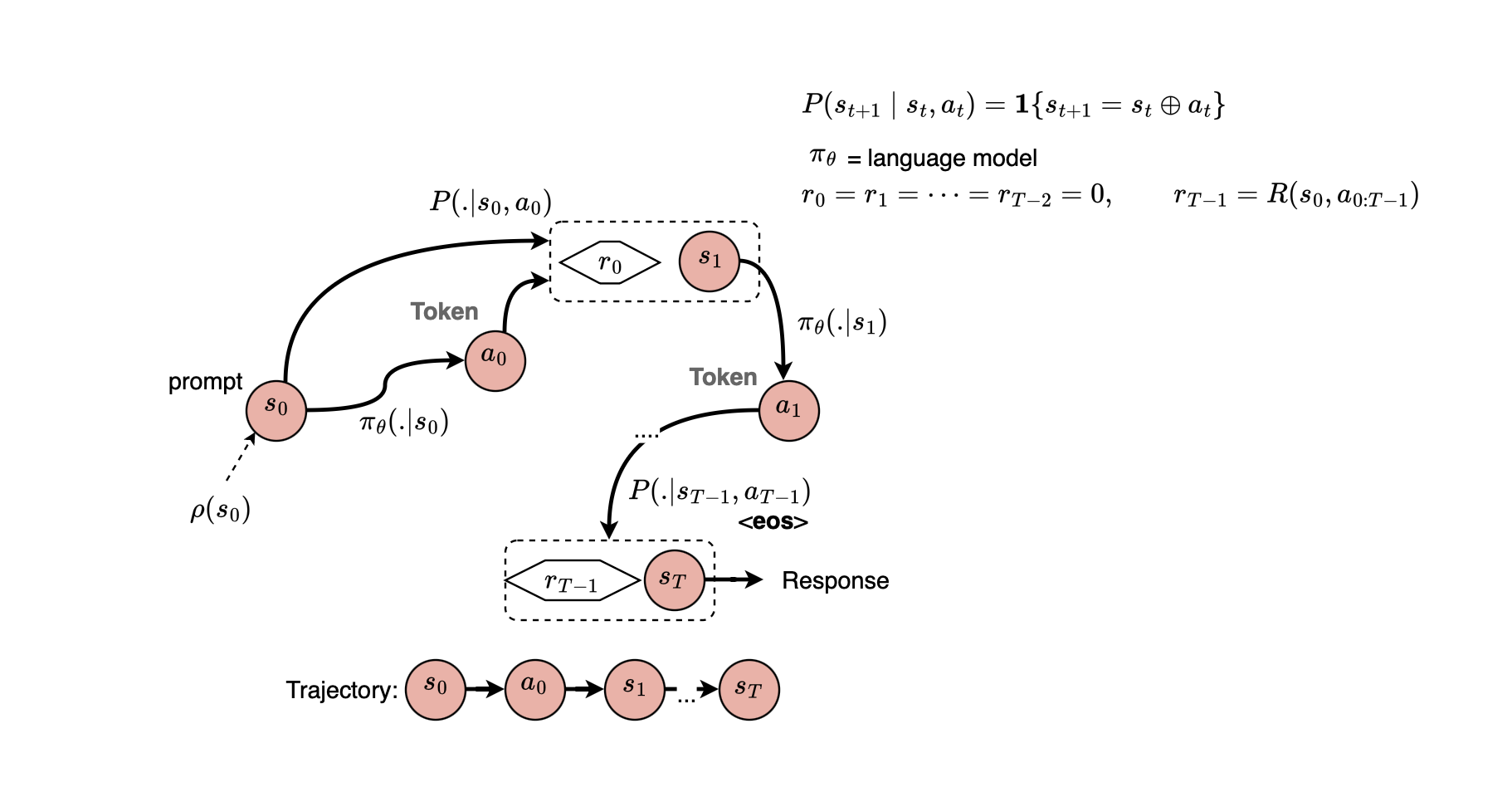
Let \(x \sim \mathbb {X}\) denote a prompt sampled from the prompt or task distribution (the prompt structure task description and instructions). Let the reward model assign a scalar reward \(R_\psi (x,y)\). In LLM reinforcement learning, the reward can be defined at the token level as
That is, the sequence-level reward is assigned when the final token is produced (or token budget reached), while the intermediate token-level rewards are \(0\). The objective is
For policy optimization, we introduce the trajectory (where each action \(a_i\) is a token sampled, that is, the action space is the set of possible output tokens)
The probability of a trajectory under the policy is
where \(\rho (s_0)\) is the initial state distribution over the prompt dataset and
is the transition probability. For an autoregressive LLM, the transition is deterministic: appending the generated token \(a_t\) to the current prefix \(s_t\) determines \(s_{t+1}\). That is,
Let the reward associated with trajectory \(\tau \) be denoted by \(R(\tau )\).
The objective becomes
We could attempt to estimate
using Monte Carlo samples,
However, after sampling the trajectories, the terms \(R(\tau ^{(i)})\) does not depend on \(\theta \). Instead, we use the log-derivative trick (we faced the same issue in VAE and instead used reparameterization trick but here we can’t):
Starting from the objective,
Moving the derivative inside,
Using
we obtain
Therefore,
From
we have
Hence,
The initial-state distribution and environment transition dynamics do not depend on \(\theta \), so
and
Therefore,
Substituting this into the policy-gradient expression gives
Using a minibatch \(\mathbb {B}\) of sampled trajectories,
Correspondingly, we can define a policy loss of the form
with the sampled trajectories treated as fixed when differentiating the Monte Carlo surrogate.
The policy gradient estimator above can have high variance. We can reduce its variance by introducing a baseline \(b(s_t)\), subtracting it from the return or empirical reward. To justify this, we first show that
Consider the complete trajectory and separate the expectation into the trajectory prefix up to \(s_t\), the current action \(a_t\), and the future trajectory:
Now,
Using
we obtain
Therefore,
Since
we have
Consequently,
Because expectation is linear,
regardless of whether the \(X_t\)’s are independent. Hence,
Thus, subtracting a state-dependent (or action independent) baseline does not change the expected policy gradient:
We can now introduce the loss
The baseline \(b(s_t)\) is typically represented using a value function,
The value function represents the expected return starting from state \(s_t\)(approximated using a deep neural network).
For state \(s_t\), the difference
acts as an advantage estimate. We therefore write
The policy objective can consequently be written in terms of the advantage as
The value network \(V_\phi \) is learned using gradient descent, separately from the policy parameters, by minimizing a mean-squared-error objective:
Now, we still have a problem with the above objective, we want to avoid large policy changes or policy degradation while reusing trajectories sampled from an older policy. We can introduce the importance sampling ratio
This leads to the surrogate objective
A KL penalty can also be added, giving an objective of the form
The reference policy \(\pi _{\mathrm {ref}}\) is generally a frozen version of the SFT policy and acts as an anchor that discourages the RL-trained policy from moving too far away from the original language model.
Finally, a clipping mechanism can be added, giving the PPO objective
where
and,
or
and
The above term is referred to as advantage estimate.
The value function is trained to minimize the prediction error between the estimated value and the observed return:
Thus, the policy is optimized using the PPO clipped surrogate objective, while the value function is trained concurrently to predict the expected return and provide the baseline used to construct the advantage. The algorithm for the PPO is listed below:
To better understand how PPO works, let’s look in detail at the implementation provided in the following article: https://cameronrwolfe.substack.com/p/llm-rl.
Given one text sample \((x,y)\), where \(x\) is the prompt and \(y\) is the generated response, let
The complete sequence is the concatenation
or with the BOS token,
After tokenization and embedding, we obtain
We pass the complete sequence \(x\circ y\) through the Transformer. Its final layer produces
Because the Transformer is causal, \(h_i\) can depend only on tokens at positions \(0,\ldots ,i\) (we can then think of \(h_i\) as compressing \((x \circ y)_{<i+1}\)). The policy model applies the language-model head to every hidden representation:
Therefore, applying the LM head to the complete hidden-state matrix gives
Here, \((x \circ y)_{<1}\) corresponds to the BOS token. Because the loss operates on the response tokens, we could write:
That is, \(x\) is the initial state of the policy, and \(h_m\) serves as a compression of the prompt for the prediction of the first response token.
The last hidden representation \(h_{m+n}\) contains the complete sequence \((x,y)\), including \(y_n\), and would be used to predict the next token \(y_{n+1}\). However, \(y_{n+1}\) is not part of the stored rollout. Therefore, the last logit is removed in the implementation:
The remaining logits are then aligned with the shifted token IDs
We do not need to physically remove the positions corresponding to the prompt \(x\). Instead, we could define the completion mask
After applying the LM head, removing the last logit, and gathering the probability corresponding to the actual next-token index at every position (from the dataset), we obtain
Applying the completion mask gives
During rollout generation, we store the log-probabilities under the policy before the PPO updates. Denote this frozen copy during the PPO optimization epochs by \(\pi _{\theta _{\mathrm {old}}}\).
Its gathered token log-probabilities are
The frozen reference model \(\pi _{\mathrm {ref}}\) similarly gives
For the rollout, the sampled per-token log-ratio relative to the reference policy (considering only \(y\)) is
In tensor form, once we apply the mask,
Now recall that the reward-to-go tensor \(\mathbf G\) introduced earlier has the form
We can build it by first multiplying the KL terms by \(-\beta \) and adding the reward to the last response token only:
We then perform a reverse torch.cumsum to obtain
The advantage is obtained by subtracting the old value estimate from the corresponding reward-to-go. For each response token,
But the value model processes the complete sequence
and, assuming it uses the hidden representations produced earlier, that is, at every position,
A scalar value head is applied independently to every hidden representation:
Therefore, the value head can compute all values in parallel through one matrix operation:
That is,
Just as with the policy logits, the final value
corresponds to the state after the final action \(y_n\) and would therefore be associated with the next action \(y_{n+1}\). Since \(y_{n+1}\) is not part of the stored rollout, this final value is not needed for the PPO loss. We therefore use
Then we could mask it:
We then obtain our advantage tensor by subtraction:
Now that we have built the advantage and reward-to-go tensor, we could start PyTorch training; that is, we use the stored token IDs produced during trajectory generation to perform a forward pass and obtain a full computation graph for all tokens in parallel in order to train the policy. We compute
That is,
We then apply clipping at the tensor level, and finally multiply the clipped and non-clipped ratios by the advantage tensor and take the minimum. We multiply by the mask again to finally produce the policy loss by taking the sum and thus produce the scalar loss presented in the algorithm listed earlier.
The critic loss is also defined by first producing the values for each token, subtracting the returns tensor produced earlier, that is, \(\mathbf G\), and taking the result to the power of \(2\). We then mask the prompt positions that are excluded from the loss and take the sum. The final loss is
Now, the above can be generalized to a batch; the only difference is that, to obtain a scalar loss, we take the mean.
Finally, we execute the backward pass and call the optimizer step to update the parameters. \(X\) epochs are performed before finishing one PPO step. In the next iteration, we set the old policy to the newly updated policy, perform the rollout again, and repeat until convergence. The reference policy \(\pi _{\mathrm {ref}}\) remains frozen.
You can now convince yourself that this is exactly what the code below does. Go through the exercise yourself; it should be very easy to follow now:
import torch

# B - batch size
# L - sequence length
# V - vocabulary size

# constants
kl_beta = 0.1
critic_weight = 0.5
ppo_eps = 0.2
num_ppo_epochs = 4

# sample completions from old policy
# compute (trajectory-level) rewards
with torch.no_grad():
    completions = policy.generate(prompts)
    rewards = reward_model(prompts, completions) # (B,)

# input_ids contains prompt + completion tokens
input_ids = torch.cat([prompts, completions], dim=-1)  # (B, L)

# causal shift
sampled_ids = input_ids[:, 1:]                   # (B, L-1)

# completion_mask: (B, L-1)
# masks out prompt and padding tokens

# get logprobs from old policy (policy that generated the rollout)
# these remain fixed during all PPO updates on this batch
with torch.no_grad():
    old_logits = policy(input_ids)               # (B, L, V)
    old_logits = old_logits[:, :-1, :]           # (B, L-1, V)

    old_per_token_logps = torch.log_softmax(
        old_logits, dim=-1
    )
    old_per_token_logps = old_per_token_logps.gather(
        dim=-1,
        index=sampled_ids.unsqueeze(-1)
    ).squeeze(-1)                                # (B, L-1)

# get logprobs of the same actions under reference policy
with torch.no_grad():
    reference_logits = reference_policy(input_ids)
    reference_logits = reference_logits[:, :-1, :]

    reference_per_token_logps = torch.log_softmax(
        reference_logits, dim=-1
    )
    reference_per_token_logps = reference_per_token_logps.gather(
        dim=-1,
        index=sampled_ids.unsqueeze(-1)
    ).squeeze(-1)                                # (B, L-1)

# compute critic values for the rollout
with torch.no_grad():
    old_values = critic(input_ids)[:, :-1]       # (B, L-1)

# compute per-token rewards
# per-token sampled KL penalty
per_token_kl = (
    old_per_token_logps - reference_per_token_logps
) * completion_mask

per_token_rewards = -kl_beta * per_token_kl      # (B, L-1)

# add outcome reward to final completion token
positions = torch.arange(
    completion_mask.size(1),
    device=completion_mask.device,
)
last_token_idx = (completion_mask * positions).argmax(dim=-1)

per_token_rewards[
    torch.arange(per_token_rewards.size(0)),
    last_token_idx
] += rewards

# compute reward-to-go / return for each token
returns = torch.flip(
    torch.cumsum(
        torch.flip(per_token_rewards, dims=[-1]),
        dim=-1,
    ),
    dims=[-1],
)                                                # (B, L-1)

# compute token-level advantages
advantages = returns - old_values                # (B, L-1)

# perform multiple PPO updates over same rollout data
for _ in range(num_ppo_epochs):

    # policy forward pass
    logits = policy(input_ids)                   # (B, L, V)
    logits = logits[:, :-1, :]                   # (B, L-1, V)

    # get logprobs of actions from current policy
    per_token_logps = torch.log_softmax(logits, dim=-1)
    per_token_logps = per_token_logps.gather(
        dim=-1,
        index=sampled_ids.unsqueeze(-1)
    ).squeeze(-1)                                # (B, L-1)

    # compute policy ratio
    policy_ratio = torch.exp(
        per_token_logps - old_per_token_logps
    )                                            # (B, L-1)

    # compute clipped policy ratio
    clipped_policy_ratio = torch.clamp(
        policy_ratio,
        min=1.0 - ppo_eps,
        max=1.0 + ppo_eps,
    )

    # compute PPO clipped policy loss
    policy_loss = -torch.min(
        policy_ratio * advantages,
        clipped_policy_ratio * advantages,
    )                                            # (B, L-1)

    # compute critic/value loss
    values = critic(input_ids)[:, :-1]           # (B, L-1)
    critic_loss = (values - returns) ** 2         # (B, L-1)

    # aggregate losses across completion tokens
    policy_loss = (
        (policy_loss * completion_mask).sum(dim=-1)
        / completion_mask.sum(dim=-1)
    ).mean()

    critic_loss = (
        (critic_loss * completion_mask).sum(dim=-1)
        / completion_mask.sum(dim=-1)
    ).mean()

    # combine policy + critic losses with critic weight
    loss = policy_loss + critic_weight * critic_loss

    # update policy and critic
    optimizer.zero_grad()
    loss.backward()
    optimizer.step()
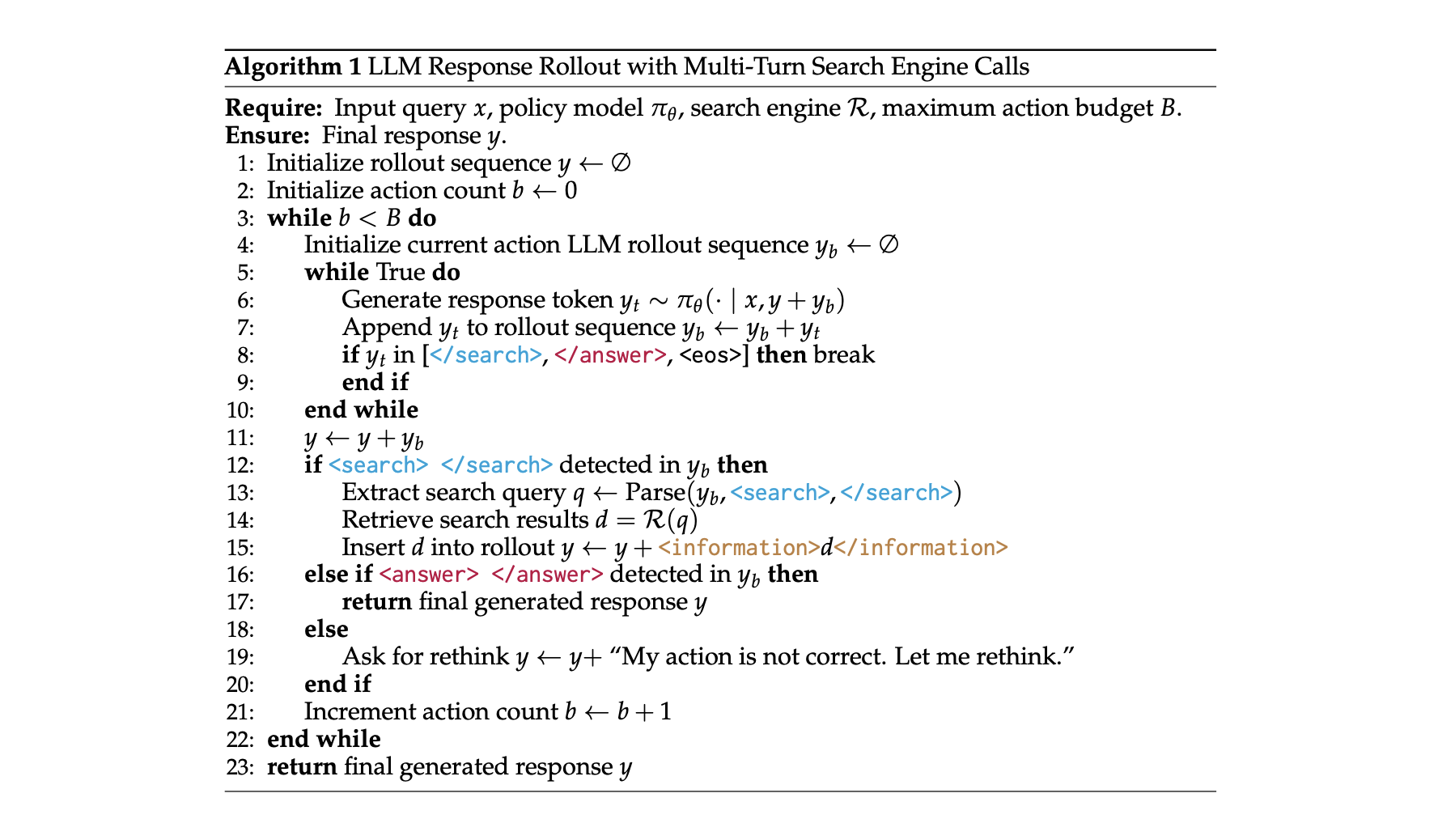
In agentic RL, the trajectory is a bit more complex than a single-step generation, as it does not merely contain LLM-generated tokens but also observations from the environment, e.g., retrieved content or the results of tool-call executions [7]. Basically, each rollout sequence is continuously parsed, and whenever a tool call (e.g a search tool) is produced by the model via special tokens, the training harness parses the tool call or tool calls, executes them, e.g., in a sandbox, and appends the resulting observations to the ongoing rollout sequence. This process continues iteratively until the maximum number of actions is reached or the model generates a final response (e.g. by producing answer special token). This is followed by reward modeling, which could use a rule-based reward system signaling whether the response is correct, or a more complex neural-based reward model, followed by updating the policy via policy-gradient methods, e.g. PPO. The policy-gradient objective is computed only over LLM-generated tokens, excluding non-LLM-generated tokens because they were not sampled from the policy, preventing interference from external content [7, 8]). However, these non-LLM-generated tokens are still part of the Transformer input, as the final answer and intermediate sub-trajectories attend to them.
Given a language model \(p_{\theta }\), during full fine-tuning, the loss is the same as in SFT:
Each model parameter \(W\) is then updated using gradient descent:
The problem is that
has the same size as \(W\), and all trainable model parameters need to be updated. Moreover, for each downstream task, full fine-tuning produces a different set of model parameters, which can be extremely large.
Instead of learning a different full \(W\) for each downstream task, LoRA or Low-rank Adapter assumes that the change in weights during model adaptation has a low intrinsic rank. It therefore learns the weight difference
such that
where
with
Only \(A\) and \(B\) are trainable; they are part of the computation graph, while \(W\) is frozen and treated as a constant. Each targeted linear projection therefore becomes
instead of simply
LoRA uses a random Gaussian initialization for \(A\) and zero initialization for \(B\). Formally, the fine-tuning objective can now be written as
where \(\theta \) denotes the frozen pretrained model parameters and \(\phi \) denotes the set of all trainable LoRA parameters \(A\) and \(B\) added to the targeted layers. Thus,
and optimization is performed only with respect to \(\phi \):
For each downstream task, only its corresponding \(\phi \) needs to be stored, while the same pretrained parameters \(\theta \) can be shared across tasks.
For an LLM, LoRA can be applied to selected linear projections in the attention and/or MLP modules. If \(L_{\mathrm {LoRA}}\) weight matrices of size \(d\times d\) are adapted with rank \(r\), the number of trainable LoRA parameters is
since each adapted matrix introduces \( |A|+|B| = rd \times dr = 2d \times r \) trainable parameters.
Observe that, in LoRA, we increase the number of model parameters and thus the memory usage. However, during the backward pass, we do not need to compute or store
for the frozen weights. Instead, we only need to compute and store
where \(A\) and \(B\) are much smaller tensors.
QLoRA is an extension of LoRA that augments the original linear projections in the same way as LoRA, while additionally quantizing the pretrained Transformer weights to 4-bit precision. Whenever a particular quantized weight or projection matrix is needed during the forward or backward pass, that tensor is temporarily dequantized to \(\mathrm {BF16}\) for the matrix multiplication. The temporary dequantized representation can then be released rather than kept permanently resident in memory, thereby reducing the memory required to fine-tune large models.
Language models, when made very large, tend to excel at new tasks unseen during pretraining. When the model is conditioned on a clear task description without any explicit examples (zero-shot learning), or on one or a few examples (few-shot learning), it seems to perform well, thereby avoiding the necessity of fine-tuning on each downstream task, which is prohibitively expensive. This is known as in-context learning, where the model, during inference, is able to generalize to new tasks conditioned on the context provided in the prompt.
Vanilla LLMs are conditioned on the prompt to produce an answer \(y_{\mathrm {answer}}\), while reasoning models produces \( y = [y_{\mathrm {CoT}}, y_{\mathrm {answer}}]\), that is, a larger trajectory that includes a thinking or Chain-of-Thought (CoT) process \(y_{\mathrm {CoT}}\), typically enclosed inside special tokens to isolate the reasoning phase before actually producing the answer. Typically, the subtrajectory corresponding to the thought process, or the non-linear reasoning traces, is hidden from the user, and a summary may be shown instead.
Naturally, training a reasoning model can be very costly, as Supervised Fine-Tuning or SFT (where the goal is to align the model’s output distribution with the data distribution) may include CoT trajectories, a high-quality set of long reasoning traces, which can be synthetically generated by strong reasoning models or manually curated, in addition to non-reasoning datasets, before RL kicks in (this is what encourages the model to produce intermediate reasoning steps at inference time, which are referred to as thinking tokens).
Again, reasoning traces are separated from the generated answers via special tokens or delimiters. For example, a fine-tuning sample could look like
Retrieval-Augmented Generation, or RAG, consists of combining information retrieval with the generative capabilities of LLMs to incorporate external knowledge (i.e., knowledge not internalized in the model parameters) and produce grounded responses (conditioned on the query and the retrieved knowledge), which can be represented as \(p_\theta (y \mid q, \operatorname {Retrieve}_k(q))\). The goal is mainly to mitigate hallucinations and build more reliable generative AI systems.
Conventional RAG operates as follows. Given a corpus of documents, each document is partitioned into chunks, and each chunk is projected into a neural embedding space. At query time, the query is also projected into the same embedding space, and the most relevant chunks are retrieved using approximate nearest-neighbor (ANN) search, optionally followed by reranking to refine the candidate selection. The retrieved chunks are then concatenated with the query to form an augmented prompt, which is provided to the LLM to generate a response.
LLMs produce a response conditioned on a given context or prompt. The response could use the internal knowledge of the language model (e.g., code generation) or answer something specific given in the prompt. In this case, the prompt could contain function-call descriptions (usually delimited using special control tokens), and the model could then produce tool or function calls according to the function schemas. This was already possible with in-context learning, but now LLMs are also trained on datasets that contain tool-use examples. The RL phase typically also teaches the model useful tool-use behaviors.
Once an LLM acquires tool-use capabilities, it can generate tool calls, and then the client or harness invoking the model reads the tool calls (what function to call and which arguments to pass to these functions), invokes them, potentially in parallel, and then injects the responses back into the context. When many LLM-based applications use the same APIs but integrate them differently, this creates fragmented integrations. Additionally, if the application cannot be modified to integrate the tools, e.g., Claude Code, then the available integrations are limited. This is why the Model Context Protocol (MCP) was introduced as a standard for tool integration, where first a standard client lists tools by communicating with an MCP server exposing the tools, and then each LLM-proposed tool call is mapped to an MCP remote call. Once the response is received, it is injected back into the context. Tool calls are what enable agents and multi-agent systems, as covered in the next section.
Finally, note that function calling opens the door to injection defects, where an adversary could redirect the model to produce malicious arguments. Thus, LLM output should be interpreted carefully (e.g., if you already know what the user ID or company ID is, form a source that you trust like jwt token, why read it again from the LLM?).
Given a system prompt describing what the model should be and which persona it should assume, the model can emit a tool call. Using the response from the tool, we can then append the result to the context or conversation history. Each request to an LLM provider is typically represented as a series of input messages, with each message having a given role. These messages are then converted into a string using a chat template and subsequently converted into tokens. This constitutes one turn.
We can create a loop and continue this process until no more tool calls are produced (enabling the model to self-reflect and self-improvement). We call this an agent, and the loop is called the agent loop. There are many optimizations for managing the conversation state, including neural retrieval and history compression, in addition to safeguards and resume handling, but the basic idea is that an agent consists of a language model, a tool set, an execution runtime, and a loop.
Given one agent, we can create a multi-agent system where intelligence gets distributed across many specialized capable subagents. Depending on the pattern used, it could consist of a parent agent delegating tasks to subagents and then combining their results to produce a response. This is called the agent-as-a-tool pattern, where each agent interaction is wrapped as a tool that the parent agent can use. In this case, the parent and subagents may or may not share conversation history. Another pattern is a handoff, where the current agent delegates control to another agent, typically using a dedicated tool, while sharing the conversation history. Alternatively, one can use a routing agent that spawns or delegates to subagents, followed by a synthesizer that combines their results. Many other patterns are possible, and the appropriate architecture depends on the problem to be solved.
Similar to how text is represented as a sequence of tokens before being fed to an autoregressive model, source code is converted into a sequence of code tokens (e.g., variable names and function names) in the same way. The model can then be trained using the same cross-entropy loss, thereby enabling code completion at inference time. That is, given a contextual prompt, the model is used to predict the code or separate code snippets that the developer is likely to write and, if equipped to do so, can autonomously add and update files. Such models can be plugged into IDEs.