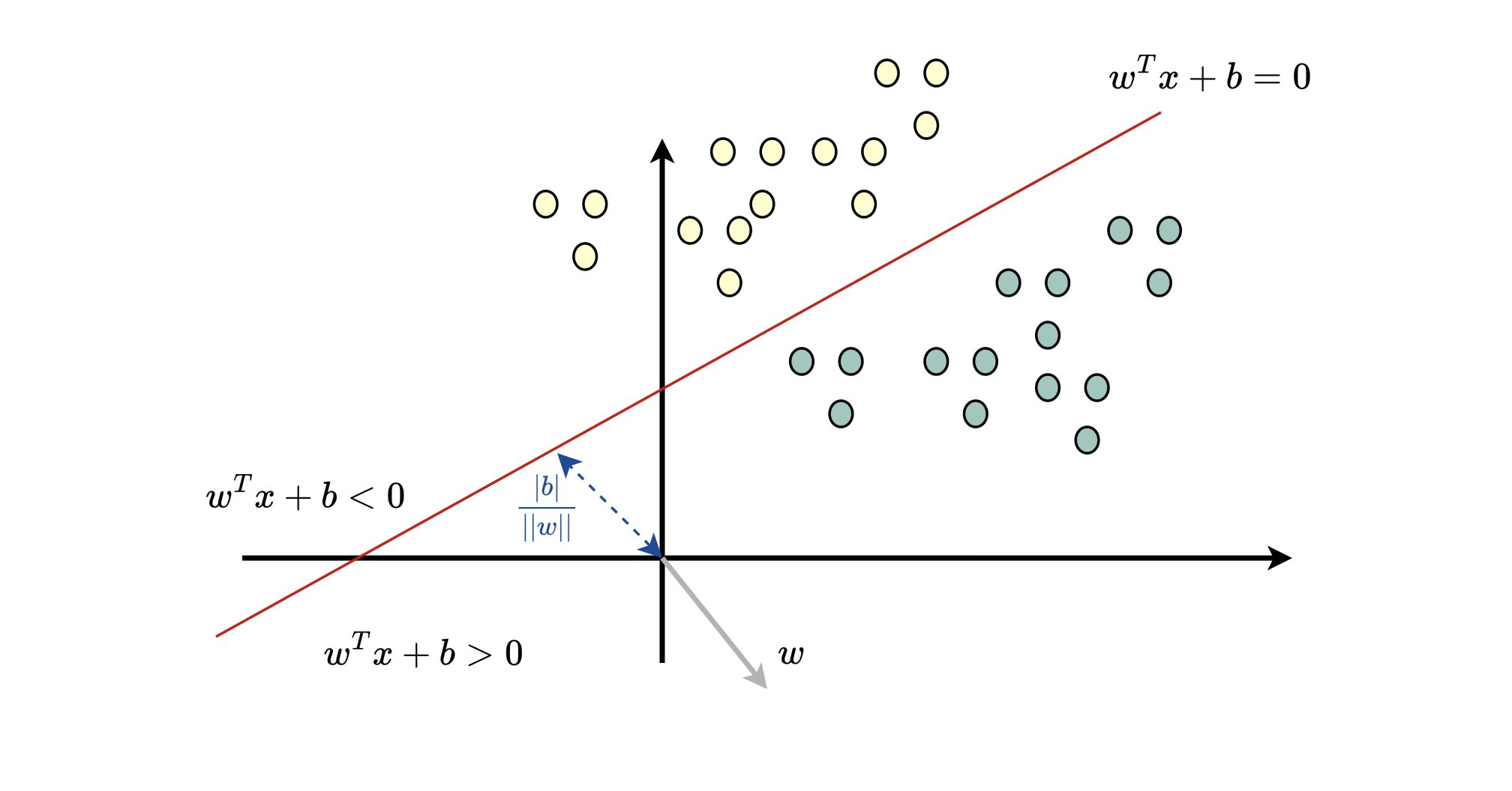
Given a dataset \( \mathbf {D} = \{(x_i, y_i)\}_{i=1}^n, x_i \in \mathbb {R}^d,\; y_i \in \{\pm 1\},\) a classifier is a function with adjustable parameters \(\theta \), \( \mathbf {f}_{\theta }: \mathbb {R}^d \rightarrow \{\pm 1\}\), that predicts the output label conditioned on \(x_i\). For example, inferring whether the behavior of a given program is malicious is a classification problem, where the label could be \(-1\) for malicious and \(1\) for benign. The goal is to have \(\mathbf {f}_{\theta }(x_i) \approx y_i\).
A linear classifier has a score of the form
Where \(\theta = \{ w,b\}\), \(b\) is the bias that shifts the decision boundary and \(w\) determines the orientation of the decision boundary (given by \(w^T x + b = 0\) ). If \(w^T x + b \geq 0\) then the predicted label is 1 otherwise -1. The classifier is then defined as
where
If a linear classifier classifies the data correctly, then the data is said to be linearly separable. More formally, a dataset is linearly separable if there exist \(w\) and \(b\), i.e., a hyperplane, such that
The minimum margin, i.e distance to closest sample, is given by:
Where we divide by \(||w||\) otherwise the projection is scaled by the size of \(w\). We multiply by \(y_i\) so that the margin is always positive for correctly classified samples, regardless of which side of the hyperplane they lie (one can also just use \(\frac {|w^T x_i + b|}{\|w\|} )\). The signed distance to the hyperplane is \(\frac {w^T x_i + b}{\|w\|}\); a negative value indicates that the sample lies on the negative side of the hyperplane. One algorithm for finding such a separating hyperplane is the Perceptron Algorithm or Gradient Ascent.
One can formulate the search for the maximum margin separating hyperplane as the following constrained optimization problem:
Given the produced score \(w^T \mathbf {x} + b\), one can turn it into a proper probability distribution using the sigmoid function:
which parameterizes the Bernoulli distribution with probability mass \(p_{\theta }(\mathbf {y} \mid \mathbf {x}) = (p_{\theta }(y = 1 \mid \mathbf {x}))^{\frac {1+y}{2}} (1-p_{\theta }(y = 1 \mid \mathbf {x}))^{\frac {1-y}{2}}\). This makes sense because \(p_{\theta }(y = 1 \mid \mathbf {x}) > \frac {1}{2}\) if and only if \(w^Tx + b> 0\).
Now, consider the scenario where we have \(L\) labels, then the classifier produces one score per class, we could write the output as \(s_{\theta }(x) = Wx + b \in \mathbb {R}^{L}\), where \(s_{\theta }(x)\) is commonly referred to as the logits. Here, the input is projected onto \(L\) different weight vectors, each with its own bias and the predicted class corresponds to the index with the highest score i.e \(\arg \max _k (Wx+b)_k\). The classifier is defined as \(\mathbf {f}_{\theta }(x) = \arg \max _{k \in \{1,...,L\}} (Wx + b)_k\). One way to learn the parameters \(W \in \mathbb {R}^{L \times d}\) and \(b \in \mathbb {R}^{L}\) is to use the Multiclass Perceptron algorithm or Gradient Ascent .
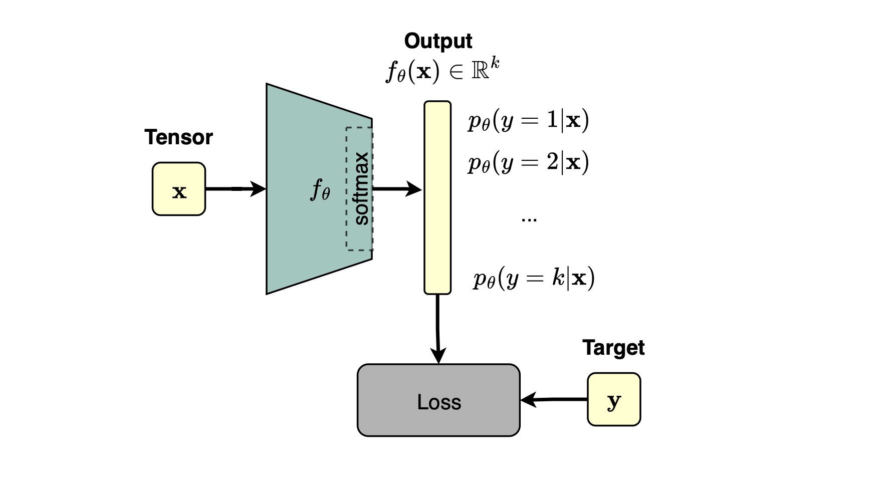
Similar to the binary case, one can turn the score function into a proper conditional distribution by using the softmax operation \( p_{\theta }(y=k \mid x) = \operatorname {softmax}(s_{\theta }(x))_k \). It makes sense because the softmax preserves ordering. The probability vector \(\pi = (\pi _1,...,\pi _L)\) where \(\pi _k:= p_{\theta }(y=k \mid x)\) and \(\sum _{k=1}^{L} \pi _k = 1\) parametrizes a categorical distribution \(\text {Cat}(y, \pi = \operatorname {softmax}(Wx+b))\) with the following probability mass function:
Now remember, we learned that we can interpret the output of a model as the parameters of a probability distribution. Later, we will see how deep neural networks are trained to learn these parameters so that the resulting conditional distribution approximates the empirical conditional distribution using maximum likelihood estimation.
Linear classification is often insufficient because its decision boundary is restricted to a hyperplane in the original input space. In many practical problems, the target classes are not linearly separable in this space. Several nonlinear transformations may therefore be required to map the input to a representation in which the classes become linearly separable. This is one of the motivations behind deep neural networks.
Deep learning consists of learning a sequence of transformations stacked together, where each layer receives the output of the previous layer, applies a linear transformation followed by a nonlinear activation function, and produces an output for the next layer. This is why it is called deep, as many layers are stacked together, and learning, because the parameters of these transformations, typically projection matrices for fully connected layers or kernels for convolutional layers, are learned from the dataset.
Binary Classification
In the field of machine and deep learning, we assume that the dataset \( \mathbb {D} = \{(x_i,y_i)\mid x_i\in \mathbb {X},\,y_i\in \mathbb {Y}\}, \) was generated through a random sampling process following unknown data distribution \(p_{\mathrm {data}}(x,y)\), that is, \((x_i,y_i)\sim p_{\mathrm {data}}(x,y)\). We do not get to know this distribution. However, we can approximate it using the empirical distribution.
The empirical joint distribution is given by
while the empirical marginal distribution of \(x\) is
Recall that in binary classification, the goal is to learn a mapping from the input space \(\mathbb {X}\) to the label space \(\mathbb {Y}\), \( f_\theta (x)\in \mathbb {Y} =\{0,1\} \).
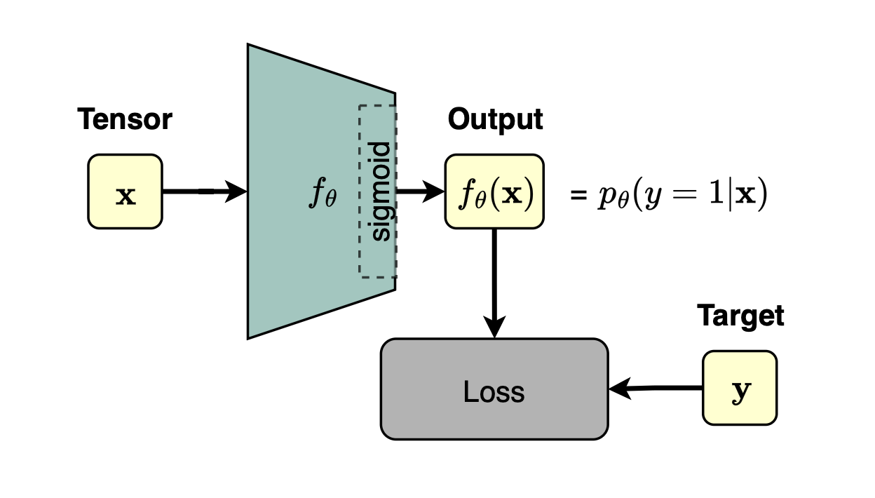
Instead of learning to map to the label directly, we will instead learn to predict, i.e interpret \(f_\theta (x)\) as \( p_\theta (y=1\mid x)\). The output of the model \(f_\theta (x)\) then parameterizes the Bernoulli distribution \(p_\theta (y\mid x)\):
or if you will
We want to find \(\theta ^{*} := \arg \min _\theta \mathbb {E}_{(x,y)\sim p_{\mathrm {\text {data}}}(x,y)} \left ( -\log p_\theta (y\mid x) \right ) = \arg \min _\theta H(p_{\text {data}}(y|x),p_{\theta }(y|x)\mathbf | p_\text {data}(x)) \)
That is, the objective function of supervised learning is to estimate the conditional (cross) entropy which measure distance between two densities. In fact, mimnimizing the cross entropy is the same as minimizing the KL divergence, which measures the discrepancy between the true conditional distribution and the model conditional distribution \(p_{\theta }(y|x)\) (as we can drop the parameter independent term), that is, \(\arg \min _\theta H(p_{\text {data}}(y|x),p_{\theta }(y|x)\mathbf | p_\text {data}(x)) = \arg \min _\theta D_{KL}(p_{data}(y|x),p_{\theta }(y|x)\mathbf | p_{\text {data}}(x) )\).
However, we do not know \(p_{\mathrm {data}}(x,y)\), so we will approximate it using the empirical distribution, that is, minimizing the negative conditional log-likelihood of the dataset \(\mathbb {D}\) (empirical cross entropy):
By the weak law of large numbers \(\mathbf {L}_{\hat {p}_{\text {data}}}(\theta )\) converges to \(\mathbb {E}_{(x,y)\sim p_{\mathrm {\text {data}}}(x,y)} \left ( -\log p_\theta (y\mid x) \right )\) and thus we can justify using the empirical negative conditional log-likelihood to estimate \(\theta ^{*}\).
Using the Bernoulli probability mass function definition,
We can define the loss (which tell us how bad the model is at prediction) as
The goal is then
where
Multiclass Classification
For multiclass classification, we parameterize a categorical distribution \(p_\theta (y\mid x)\).
The model produces a vector of scores followed by a softmax, resulting in
where \(K\) is the number of classes and
The categorical distribution can be written as
We want to find
As in the binary case, this corresponds to minimizing the conditional cross-entropy
Since
and the first term does not depend on \(\theta \), minimizing the conditional cross-entropy is equivalent to minimizing the conditional KL divergence. However, again we do not know \(p_{\mathrm {data}}(x,y)\), so we approximate it using the empirical distribution. We obtain the MLE
Using the categorical probability mass function,
For each sample, the inner term can also be written as
The loss can then be formulated as
For the empirical conditional distribution,
and therefore we can equivalently write
By the weak law of large numbers, for a fixed \(\theta \),
Deep learning models can broadly be divided into two categories: discriminative models and generative models. Discriminative models learn the conditional distribution \(p_\theta (y \mid x)\), where \(x\) denotes the input and \(y\) the corresponding target. The objective is to approximate the unknown data distribution \(p_{\text {data}}(y \mid x)\). For example, in binary classification, the output of the neural network is interpreted as the parameter of a Bernoulli distribution, as covered earlier, \(p_\theta (y=1\mid x)=f_\theta (x)\) where \(f_\theta (\cdot )\) denotes the deep neural network. Given training samples \(\{(x_i,y_i)\}\) assumed to be sampled from the unknown distribution \(p_{\text {data}}(x,y)\), the model is typically trained by minimizing the cross-entropy loss, which is equivalent to maximizing the likelihood of the observed labels or, equivalently, minimizing the KL divergence between the true conditional distribution \(p_{\text {data}}(y\mid x)\) and the model distribution \(p_\theta (y\mid x)\). The empirical cross-entropy converges in probability to the conditional cross-entropy as the number of samples increases (\(n\rightarrow +\infty \)).
Generative models, on the other hand, learn how the data itself is generated by approximating the data distribution \( p_{\text {data}}(x) \). For example, Generative Adversarial Networks or GANs learn an implicit distribution by mapping samples drawn from a simple prior distribution \(p(z)\), typically a standard Gaussian, through a generator network \(G_\theta (z)\). On the other hand, Variational Autoencoders or VAEs explicitly introduce a latent variable \(z\) and model the joint distribution \( p_\theta (x,z)=p_\theta (x\mid z)p(z)\), where \(p(z)\) is a predefined prior, usually a standard Gaussian. The data likelihood is then given by \( p_\theta (x) = \int p_\theta (x\mid z)p(z)\,dz, \) which is generally intractable to compute exactly. Large Language Models or LLMs are also generative models. They learn the joint probability distribution of a sequence of tokens by factorizing it using the chain rule (autoregressive or AR modeling), \( p_{\theta }(x_1,\ldots ,x_n) = p_{\theta }(x_1) \prod _{i=2}^{n} p_{\theta }(x_i\mid x_1,\ldots ,x_{i-1}). \). Training consists of learning each conditional distribution so that the model can accurately predict the next token given all previous ones (which is easier than generating celebrity faces). Once trained, the model can either compute the likelihood of a sequence or generate new text by repeatedly sampling or selecting the next token from the learned conditional distribution.
In the field of deep learning, we assume that the data was generated from some unknown distribution (i.e there is a data-generating process behind), and we attempt to approximate it using a parametric model \(p_\theta (x)\). We observe random samples \(\{x_i\}_{i=1}^n\) where \(x_i \sim p_{\text {data}}(x)\) (the datapoints are assumed to be iid). The goal of learning is to find \(\theta \) such that \(p_\theta (x) \approx p_{\text {data}}(x)\) i.e., we approximate the underlying data distribution (using the empirical distribution). Once we have learned \(p_\theta (x)\), we can generate artificial or synthetic samples. However, under the manifold hypothesis, \(p_{\text {data}}(x)\) is concentrated on a low-dimensional manifold embedded in a very high-dimensional ambient space. This motivates introducing a lower-dimensional latent space from which the observed data can be generated.
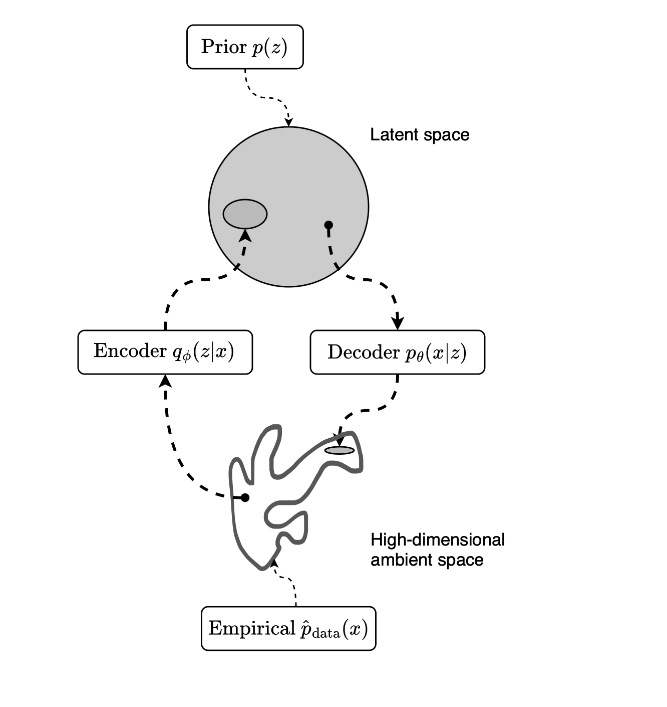
We learn how to transform a simple fixed distribution in latent space, for example \(p(z)=\text {Normal}(0,I)\), into the data distribution. Rather than learning a mapping as in GANs, we use conditional modeling and learn the conditional density \(p_\theta (x \mid z)\). More precisely, we model
To estimate \(p_{\text {data}}(x \mid z)\), we use a deep neural network whose output parameterizes the conditional distribution \(p_\theta (x \mid z)\) (i.e., the decoder parameterizes this distribution). We assume that the observed data were generated from latent variables, i.e., pairs \((x,z)\) were generated, but only \(x\) is observed while \(z\) remains hidden.
Since \(x\) and \(z\) are dependent, we can write the marginal likelihood as (assuming the prior is fixed and known)
Our objective is to learn \(\theta \) such that
Unfortunately, \(p_\theta (x)\) intractable (i.e no analytic solution) because \(p_\theta (x\mid z) = \mathcal {N}\!\left (x;f_\theta (z),\sigma ^2 I\right )\) is parameterised using a multi-layer neural-network decoder, making the integral impossible to evaluate analytically. We could use naive Monte Carlo estimation by sampling a large number of latent variables from the prior \(z_k \sim p(z)\) and compute \(p_\theta (x)\) approximately
Giving
While writing the marginal likelihood as an expected value with respect to the prior distribution seems to solve the problem, it leads to an unstable estimator, as most of the sampled \(z\) values will result in likelihood values close to zero. We are likely to miss, by chance, those samples that would result in high likelihood values, thereby increasing the variance of the estimator (very large random samples are needed) [?, ?]. To see why, imagine drawing latent vectors from the prior. For a given observation \(x\), only a small subset of latent variables \(z\) are likely to explain it well. Consequently,\( p_\theta (x\mid z)\approx 0\) for most sampled \(z\). By Bayes’ rule,
this implies that the posterior places almost all of its probability mass on a very small region of the latent space, while assigning nearly zero probability to the rest.
The key idea behind Variational Autoencoder or VAE is therefore to introduce an approximate posterior distribution \(q_\phi (z\mid x)\) to produce latent variables that are likely to assign a high probability to the observation through \(p_\theta (x\mid z)\). This provides an efficient way to identify the regions of latent space that explain the data and serves as the first step toward learning a latent representation that can later be used for generation by sampling from the prior.
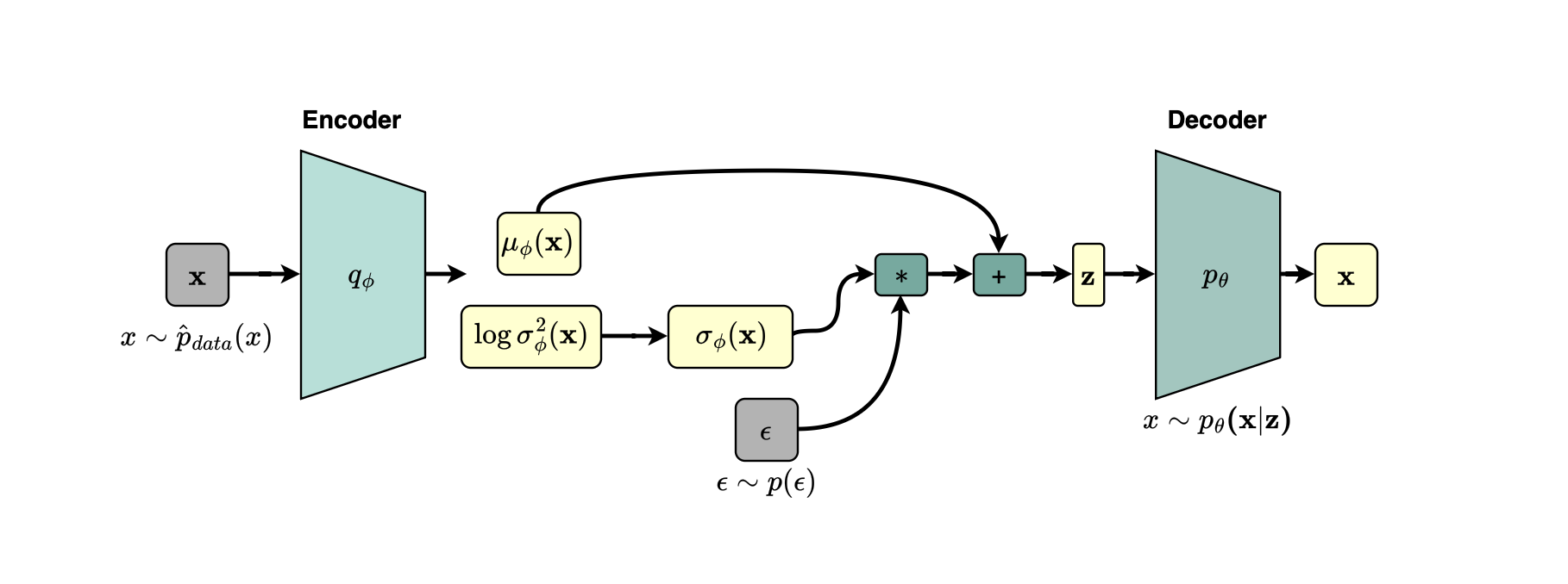
We start from the marginal likelihood
and therefore
Introducing an arbitrary distribution \(q(z)\), we can write
or,
Taking the expectation with respect to \(q(z)\),
Since \(\log p_\theta (x)\) does not depend on \(z\),
Using
we obtain
Expanding the first term gives
Since
we obtain
Therefore,
because
The term
is known as the Evidence Lower Bound or ELBO for short.
We now set
where \(q_\phi (z\mid x)\) is parameterized by an encoder with parameters \(\phi \).
The VAE objective becomes
For the empirical data distribution,
where the expectation over \(q_\phi (z\mid x_i)\) can be approximated using Monte Carlo sampling.
We assume that \(q_\phi (z\mid x)\) parameterizes a Gaussian distribution.
For a latent space of dimension \(b\),
Equivalently,
The encoder therefore outputs
or, in practice, typically
Assume the prior is
Then the KL divergence has a closed-form expression:
Therefore,
Hence, the loss can be simplified to
Now we need to to compute \( \frac {\partial \mathbf {L}}{\partial \theta } \qquad \text {and}\qquad \frac {\partial \mathbf {L}}{\partial \phi }\). Computing the gradient with respect to \(\theta \) is simple because we can use Monte Carlo sampling to eliminate expectation \(\mathbb {E}_{q_\phi (z\mid x_i)}\).
For example,
But what about \( \frac {\partial \mathbf {L}}{\partial \phi }\)
This is a little problematic because the distribution from which we sample depends on \(\phi \).
In general,
For the second term,
the closed-form expression depends explicitly on \(\phi \), and its gradient can be obtained using automatic differentiation.
The remaining problem is therefore how to compute
Instead, we use the reparameterization trick.
We write
We can therefore write
Then
The randomness has now moved from \(z\) to \(\epsilon \), whose distribution \( p(\epsilon )=\mathcal {N}(0,I)\) does not depend on \(\phi \). Consequently,
Since \(p(\epsilon )\) does not depend on \(\phi \), we can move the derivative inside the expectation:
We can now use Monte Carlo sampling. Observe that \(p_\theta (x\mid z)\) depends on \(\phi \) through \( z = \mu _\phi (x) + \sigma _\phi (x)\odot \epsilon \). For example, if the decoder distribution \(p_\theta (x\mid z)\) is Gaussian, the reconstruction term can correspond to an \(L_2\) loss.
We can therefore write the VAE objective as
Using a single Monte Carlo sample
we obtain
and the objective becomes
This objective is then trained using SGD.
GANs, or Generative Adversarial Networks (and many other generative and machine learning models like diffusion models or autoencoders) are motivated by the manifold hypothesis concept, which states that the data of interest (e.g natural images or celebrity faces) form a thin d-dimensional submanifold \(\mathbb {M}\) embedded in a high-dimensional ambient space \(\mathbb {X}\) (e.g \(\mathbb {R}^D\), where \(d<D\); d is known as intrinsic dimension while \(D\) is the ambient dimension).
GAN tries to learn a mapping from a given latent space \(\mathbb {Z}\) to \(\mathbb {M}\) and then samples from \(\mathbb {M}\) by sampling from \(\mathbb {Z}\).
In GAN, there is no explicit likelihood maximization as in a VAE (i.e it is not a likelihood-based model). Instead, there is a generator \(g_\theta (z)\) that generates a candidate sample \(x_{\text {fake}} = g_\theta (z)\), where \(g_\theta \) is a deep neural network.
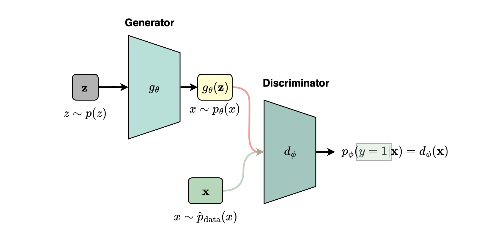
The generator is trained to fool a discriminator (binary classifier) \(d_\phi \) in an adversarial fashion. The discriminator, represented by \(d_\phi \), outputs the probability that a sample is real. The goal of the discriminator is to maximize \(\log d_\phi (x)\) for real samples \(x \sim p_{\text {data}}\), and to maximize \(\log \left (1-d_\phi (g_\theta (z))\right )\) for fake samples \(z \sim p(z)\).
The loss is the standard binary cross-entropy loss (i.e., similar to training a binary classifier) and is given by (which is equivalent to minimizing the Jensen-Shannon divergence)
As usual, we do not have access to the true data distribution, and thus we approximate it using the empirical distribution:
The term \(\mathbb {E}_{z\sim p(z)}\) is approximated using Monte Carlo sampling. During SGD training, when training the discriminator, the generator parameters are kept fixed, i.e., the generator does not learn. Similarly, when training the generator, the discriminator parameters are kept fixed. With PyTorch, this alternating training procedure is straightforward to implement.
Getting a GAN to work can be difficult due to vanishing gradients, non-convergence, instability of the adversarial equilibrium, and especially mode collapse. Mode collapse can happen when the generator learns a distribution concentrated on only a few modes or examples instead of approximating the full data distribution.