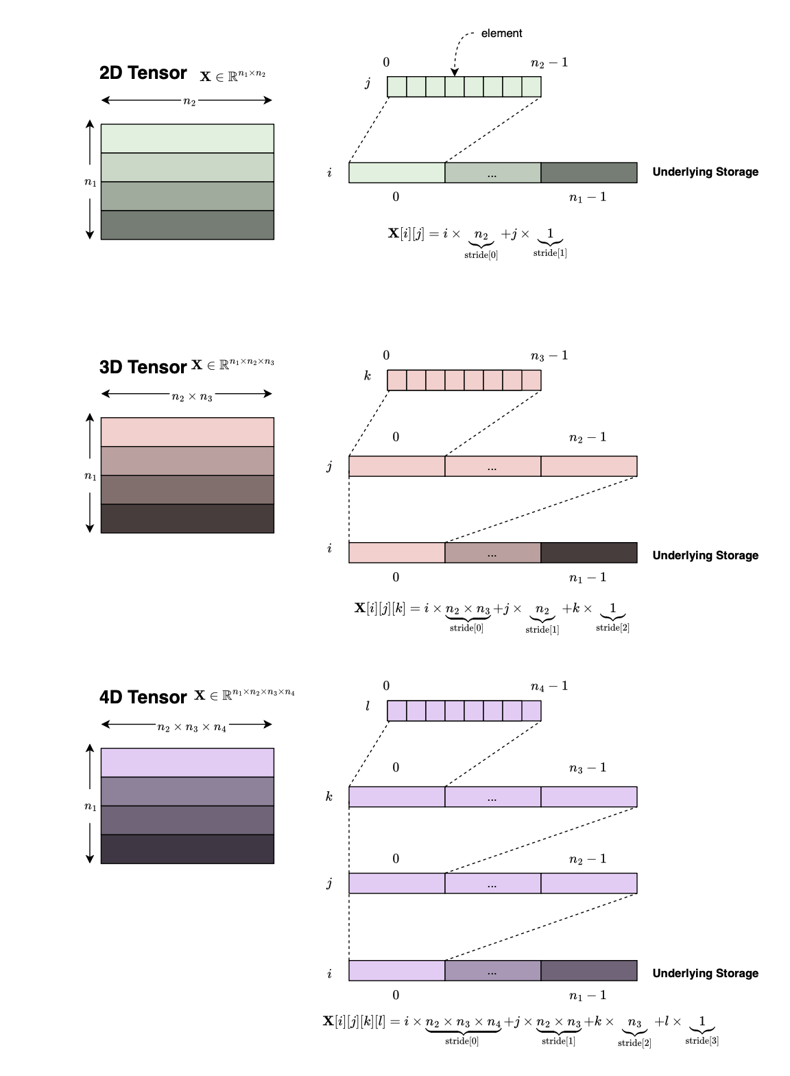
Tensors are fundamental data structures in Torch. Before we discuss how tensors are represented, let us first understand how a high-dimensional array is physically stored in memory, that is, how, given a multi-dimensional tensor index, we can compute its address in memory.
If the dimension of the ambient space is \(1\), then the array reduces to a single scalar. Such a scalar may occupy, for example, \(8\) bytes (\(64\) bits). In many cases, the compiler stores local scalar variables directly on the stack for efficiency rather than allocating memory on the heap.
Now consider a two-dimensional array containing \(M \times N\) elements. There are two common ways to lay out such an array in memory, row-major order and column-major order. In a row-major layout, all the elements of the first row are stored contiguously in memory, followed by all the elements of the second row, and so on.
Assuming each element occupies one byte (the smallest addressable unit), the memory address of the element \(\mathbf {A}(i,j)\) is
where \(\operatorname {offset}\) denotes the base address of the array in memory.
More generally, consider an \(n\)-dimensional array whose size along dimension \(k\) is denoted by \(s_k\). The row-major layout defines a mapping
which maps an index or iteration vector
to a linear memory address or offset according to
Thus, the memory address of an element of the array \(\mathbf {A}\) can be written as
Rather than repeatedly computing these products, it is convenient to introduce the notion of strides, which tell us how many memory elements we need to cross to move from one index to the next along a particular dimension. The stride of dimension \(i\) is defined as
with the convention that
For example,
Using the stride array, the memory address becomes much simpler:
The multidimensional array \(\mathbf {A}\) described above is precisely what is commonly referred to as a tensor. A tensor is therefore nothing more than a multidimensional array together with enough metadata to interpret its underlying storage.
One consequence of the stride representation is that many tensor transformations require no data movement. Consider the transpose of a two-dimensional tensor. Originally, the address computation is
After transposition, we simply exchange the strides (instead of physically rearranging the data, we just swap the strides from \((N,1)\) to \((1,N)\), although cache locality may no longer be enjoyed):
The underlying storage remains unchanged. This is why a PyTorch tensor view can avoid materializing the transposed tensor.
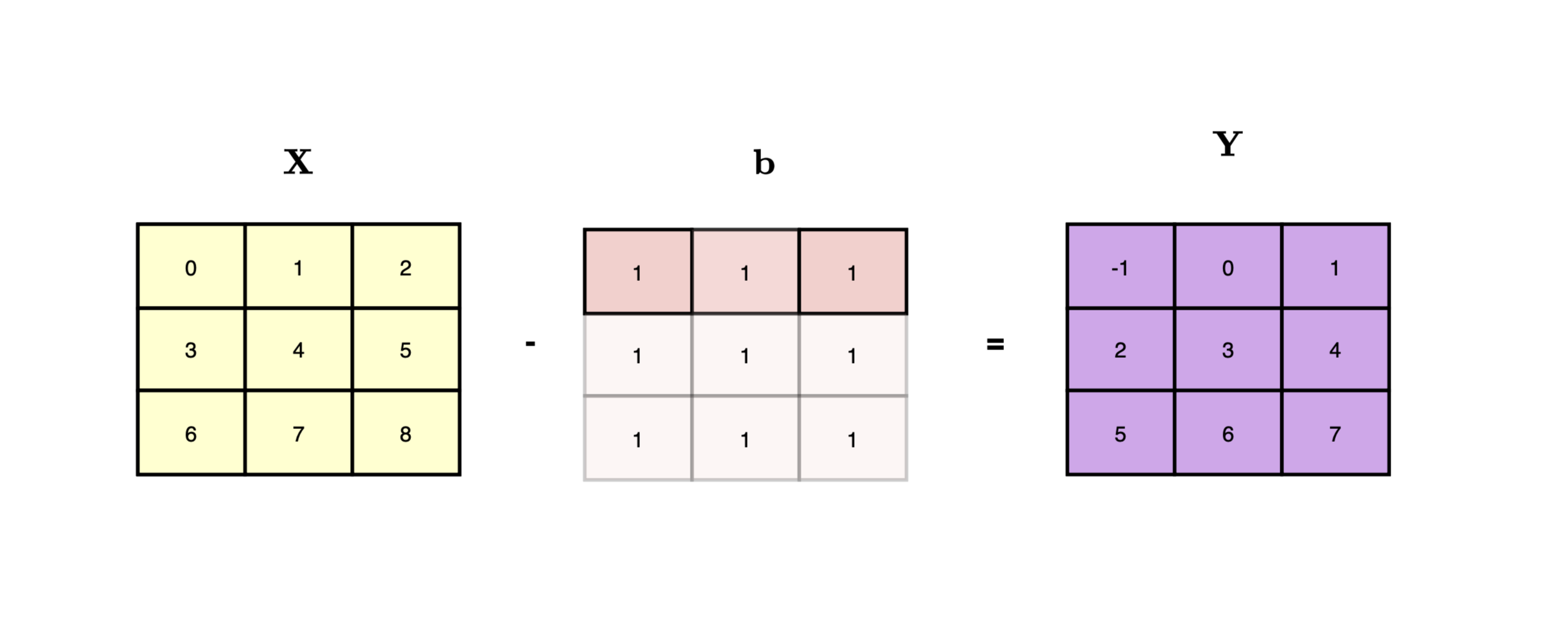
Another benefit of using a stride-based representation is broadcasting. For example, when using TensorIterator, PyTorch computes the broadcasted shape, allowing us, for example, to subtract two tensors \(\mathbf {X}\) and \(\mathbf {b}\), with \(\mathbf {X} \in \mathbb {R}^{n \times m}\), i.e., \(\operatorname {shape}=[n,m]\), and \(\mathbf {b} \in \mathbb {R}^{m}\), i.e., \(\operatorname {shape}=[m]\). Instead of copying \(\mathbf {b}\) into a new tensor, we can define a new view of \(\mathbf {b}\) using the same underlying storage, but with \(\operatorname {shape}=[n,m]\) and \(\operatorname {stride}=[0,1]\). The zero stride means that, when moving along the first dimension, we always read the same vector again for each point in the iteration space.
A key data structure in PyTorch is the Tensor object. Gradients are tensors, inputs are tensors, and even the loss is represented as a tensor.
A tensor can be created directly, for example by calling torch.rand(), or produced as the result of a tensor operation such as matrix multiplication or addition.
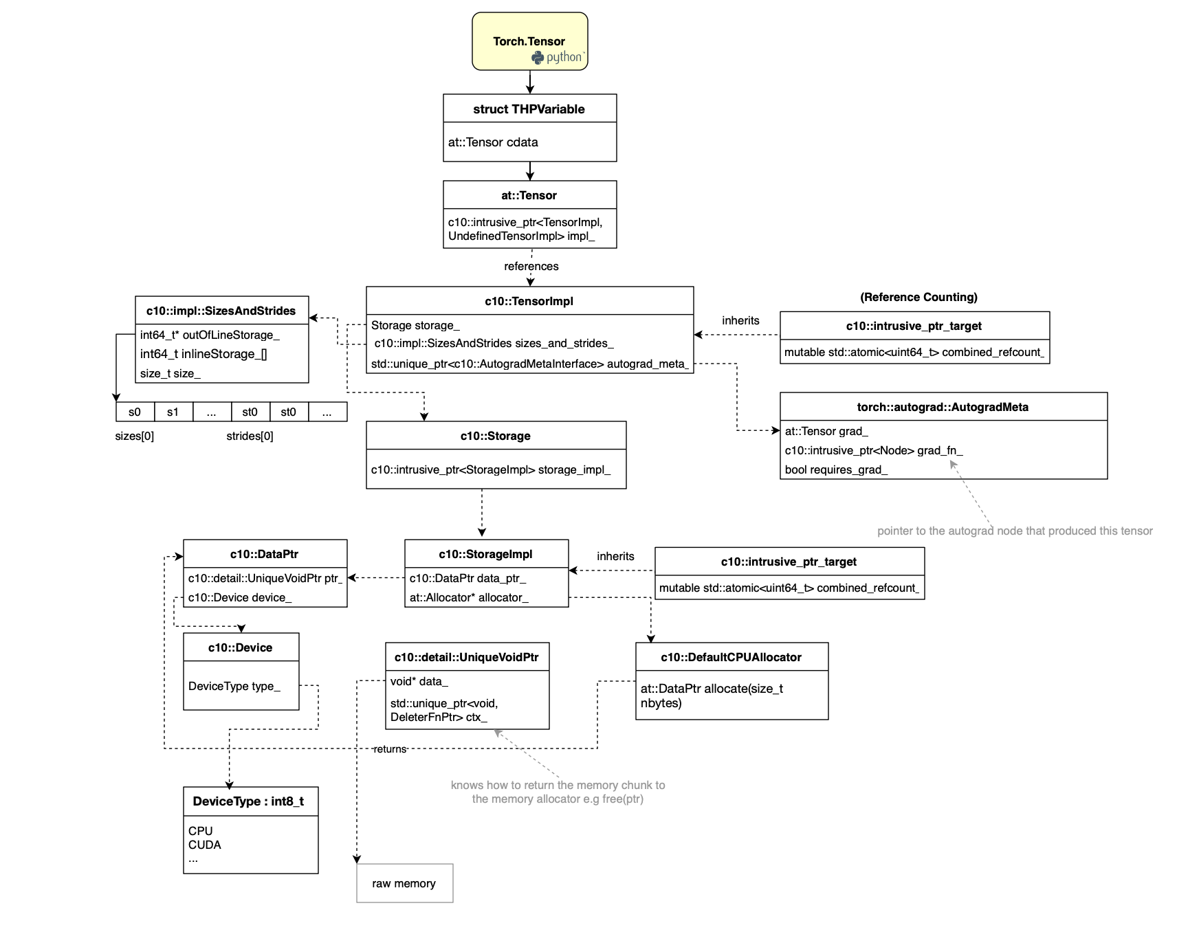
When you create a Python tensor object, the torch.Tensor object is represented internally by a THPVariable instance. As depicted below, THPVariable wraps the C++ Tensor, which knows how to access underlying data and dispatching tensor operations.
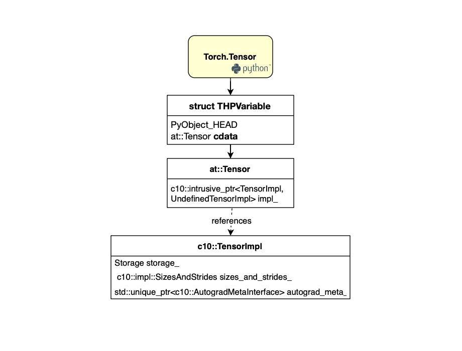
Each Tensor object actually holds a reference to the underlying tensor implementation, TensorImpl. This implementation stores the tensor metadata, including its rank, the size of each dimension, the strides, and the storage offset, all of which are used to compute the virtual memory address corresponding to a given index.
To enable data sharing without expensive copies, TensorImpl owns a Storage object, which in turn references a shared StorageImpl containing a pointer to the actual allocated memory.
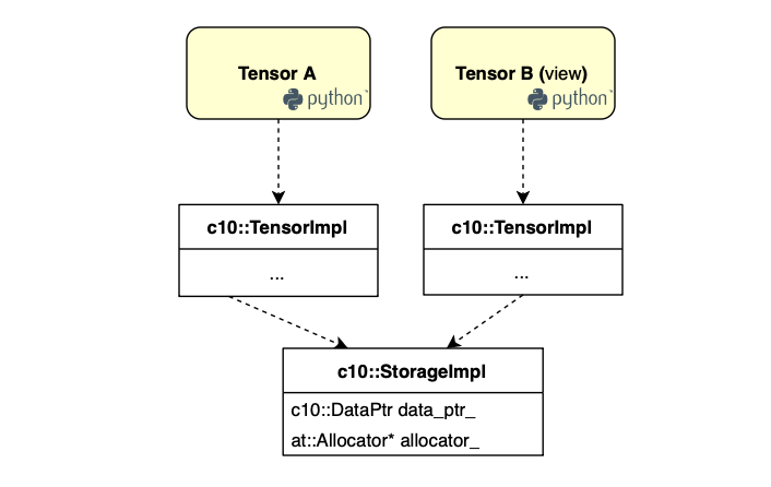
The tensor data can be allocated on the CPU or on another device such as a GPU. When the tensor resides on the CPU, PyTorch uses the DefaultCPUAllocator, which may rely on an underlying allocator such as mimalloc to perform the actual memory allocation.
Finally, TensorImpl holds a pointer to an AutogradMeta structure, which stores autograd-specific information such as the tensor’s gradient, the tensor (grad_fn), and other metadata required for automatic differentiation.
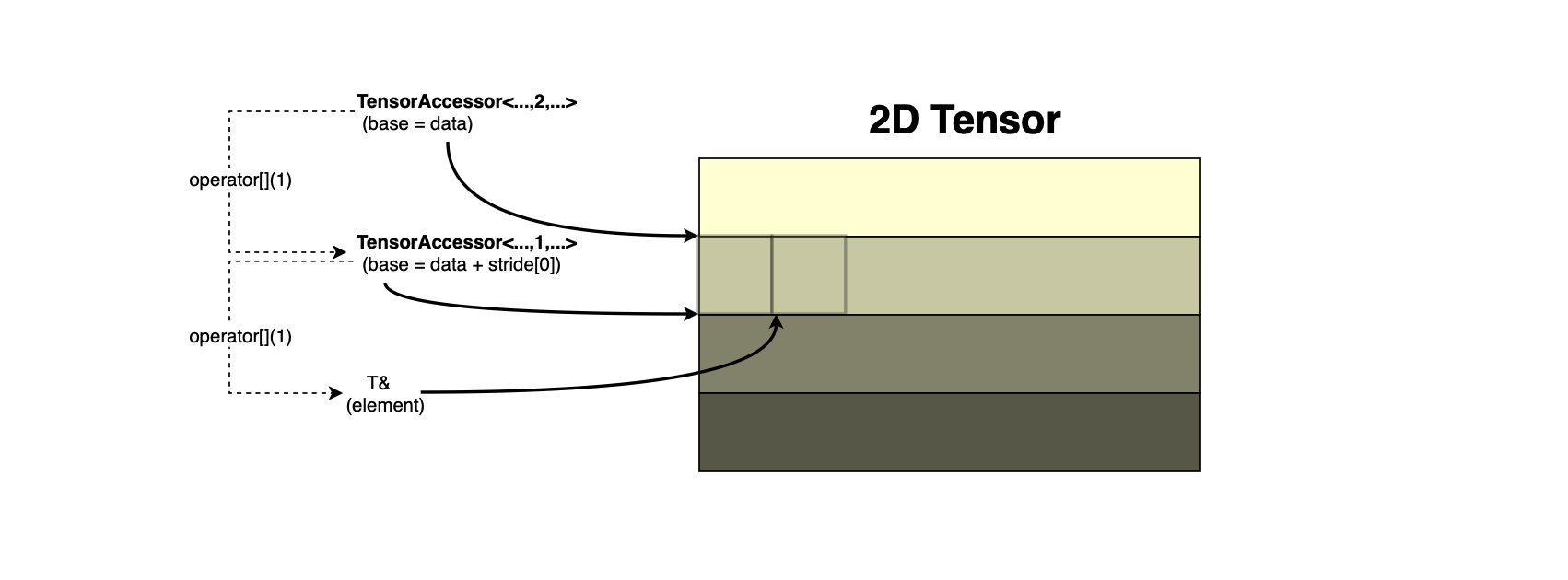
Accessing tensor data can be facilitated using TensorAccessor, which advances its base pointer
each time the subscript operator is invoked. Specifically, the index is multiplied by the stride of the
current dimension, and a new TensorAccessor is created unless the last dimension is reached (i.e.,
the rank is 1). In that case, the subscript operator returns a reference to the actual tensor
element. This is implemented using C++ templates, one specialization is provided for
TensorAccessor
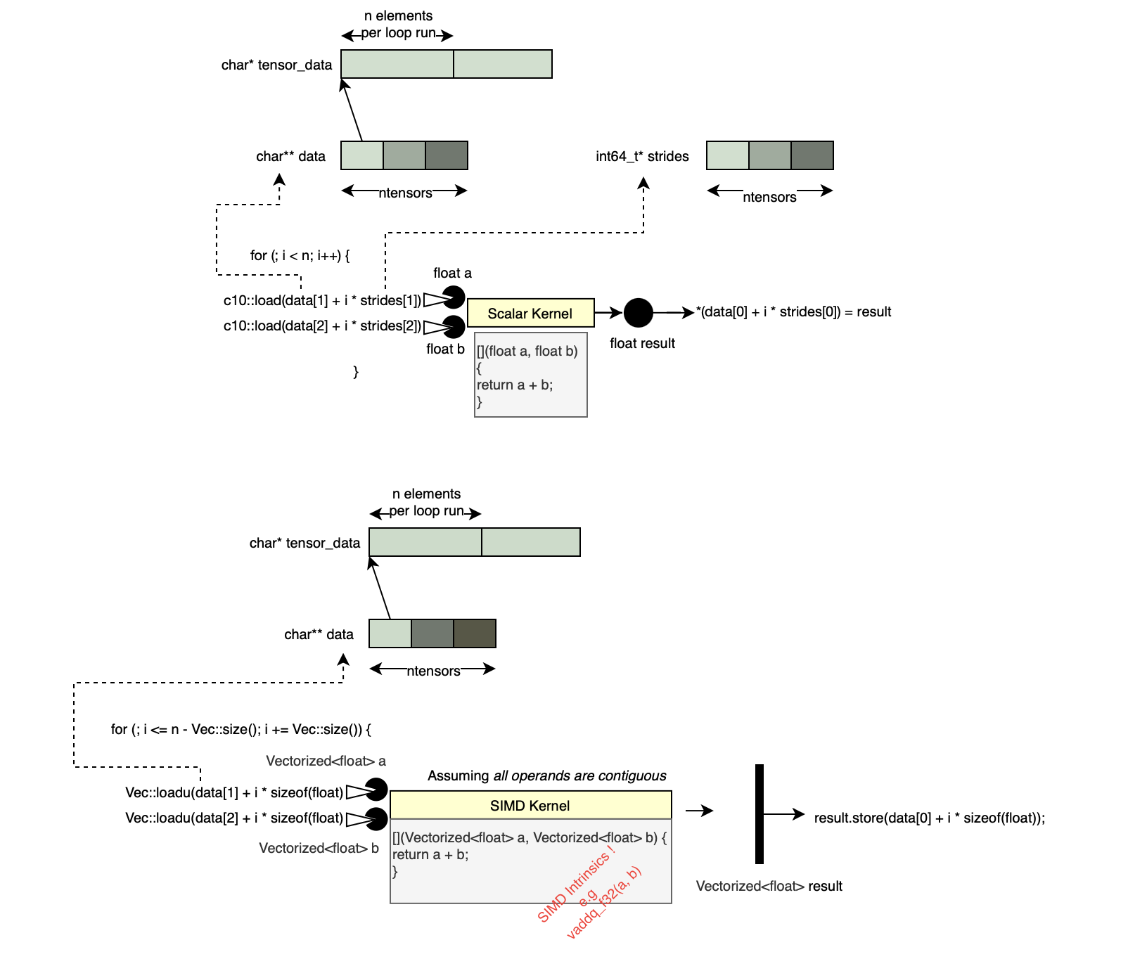
TensorIterator enables defining either a scalar kernel to be applied over one or more operands. Under the hood, PyTorch sets up the base data pointers for the input and output operands, handles parallelization across the iteration range, and performs the necessary pointer arithmetic. This greatly improves code reuse. Additionally, TensorIterator supports vectorized kernels, which exploit SIMD vector hardware.
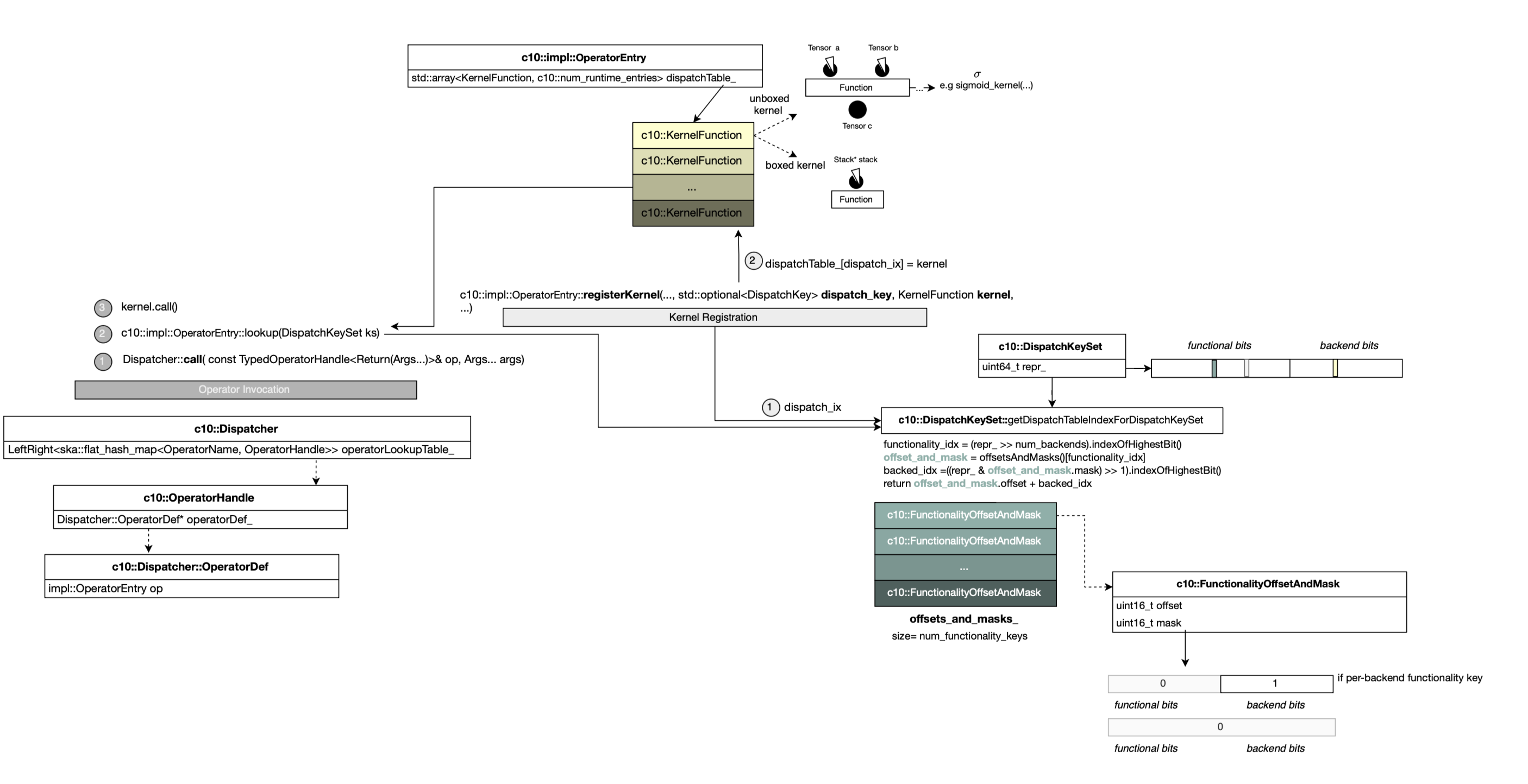
Torch defines a large set of kernels that operate on tensors and produce another tensor as the result of an operation, such as addition. Specifically, there are two types of kernel functions. Boxed kernels are generic kernels that receive a stack of values (IValue) and can inspect or manipulate the stack (e.g., Python fallbacks). In contrast, unboxed kernels are regular C++ functions, such as a sigmoid kernel, whose argument types are known ahead of time.
Kernels are invoked through the dispatching mechanism. Each kernel is registered for a particular dispatch key, which identifies both the functionality and the backend implementation. For example, the addition operator for dense CPU tensors corresponds to the CPU dispatch key. Whenever the dispatcher is invoked to execute an operator such as sigmoid, it first consults its lookup table to retrieve the corresponding operator handle.
  const KernelFunction& lookup(DispatchKeySet ks) const {

    # Find the highest index in the dispatch table in OperatorEntry
    const auto idx = ks.getDispatchTableIndexForDispatchKeySet();
    ....
    const auto& kernel = dispatchTable_[idx];
    ...
    return kernel;
  }
The operator handle refers to an operator entry, which stores the registered kernels for every dispatch key. The operator entry then computes the dispatch index, i.e., determines the highest-priority dispatch key from the dispatch key set, indexes into the dispatch table, and finally invokes the selected kernel.
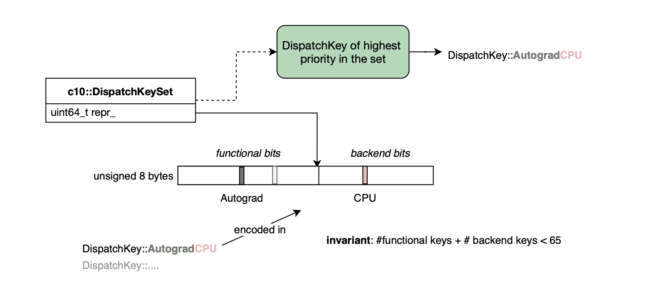
Once a kernel is invoked, it may remove its own dispatch key from the dispatch key set and redispatch the operation. For example, during tensor addition, the AutogradCPU kernel is invoked first. It creates the autograd node required for backpropagation and gradient computation, then redispatches the operation after removing the AutogradCPU dispatch key from the dispatch key set. The CPU kernel is then selected, performs the actual addition, and returns the resulting tensor. Control then returns to the autograd kernel, which saves any information required for the backward pass before returning the final result.
Almost every tensor operation goes through the dispatcher, including memory allocation. Whenever the dispatcher is invoked, it first constructs a dispatch key set by inspecting the arguments (e.g., the dispatch keys carried by tensor arguments).
template <class Return, class... Args>
C10_ALWAYS_INLINE_UNLESS_MOBILE Return Dispatcher::call(
    const TypedOperatorHandle<Return(Args...)>& op,
    Args... args) const {
  # Inspect arguments and infer the dispatch key set
  auto dispatchKeySet =
      op.operatorDef_->op.dispatchKeyExtractor()
          .template getDispatchKeySetUnboxed<Args...>(args...);
  ...

  # look up the kernel
  const KernelFunction& kernel = op.operatorDef_->op.lookup(dispatchKeySet);
...

  # invoke the kernel
  return kernel.template call<Return, Args...>(
      op, dispatchKeySet, std::forward<Args>(args)...);
}
This dispatch key set is then used to determine which kernel should execute. In some cases, however, there is insufficient information to determine the backend directly, such as during memory allocation. In these situations, the special BackendSelect dispatch key is used to inspect the arguments, infer the appropriate backend, and redispatch the operation with the updated dispatch key set. This entire process is illustrated below.
native_functions.yaml defines which operators exist and which kernels implement them. It is primarily responsible for defining forward operators and their dispatch. For example:
- func: add.Tensor(Tensor self, Tensor other, *, Scalar alpha=1) -> Tensor
  device_check: NoCheck   # TensorIterator
  structured_delegate: add.out
  variants: function, method
  dispatch:
    SparseCPU, SparseCUDA, SparseMPS, SparseMeta: add_sparse
    SparseCsrCPU, SparseCsrCUDA, SparseCsrMeta: add_sparse_csr
    MkldnnCPU: mkldnn_add
    ZeroTensor: add_zerotensor
    NestedTensorCPU, NestedTensorHPU, NestedTensorCUDA: NestedTensor_add_Tensor
  tags: [core, pointwise]
On the other hand, derivatives.yaml tells Autograd how to differentiate operators by specifying their backward formulas (PyTorch will generate the C++ code for the derivatives during the build time). For example, for multiplication:
- name: mul.Tensor(Tensor self, Tensor other) -> Tensor
  self: mul_tensor_backward(grad, other, self.scalar_type())
  other: mul_tensor_backward(grad, self, other.scalar_type())
  result: other_t * self_p + self_t * other_p
For the sigmoid operator:
- name: sigmoid(Tensor self) -> Tensor
  self: sigmoid_backward(grad, result)
  result: auto_element_wise