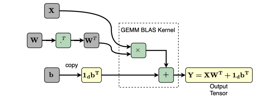
A linear layer consists of multiplying the input tensor \(\mathbf {X} \in \mathbb {R}^{d \times n}\) by a weight matrix \(\mathbf {W} \in \mathbb {R}^{m \times n}\) and then adding a bias vector \(\mathbf {b} \in \mathbb {R}^{m}\) to produce an output tensor \(\mathbf {Y} \in \mathbb {R}^{d \times m}\) (this means that the new representation has dimension \(m\) instead of \(n\)). In matrix form, it can be written as
For a single sample \(\mathbf {x} \in \mathbb {R}^{n}\), this becomes
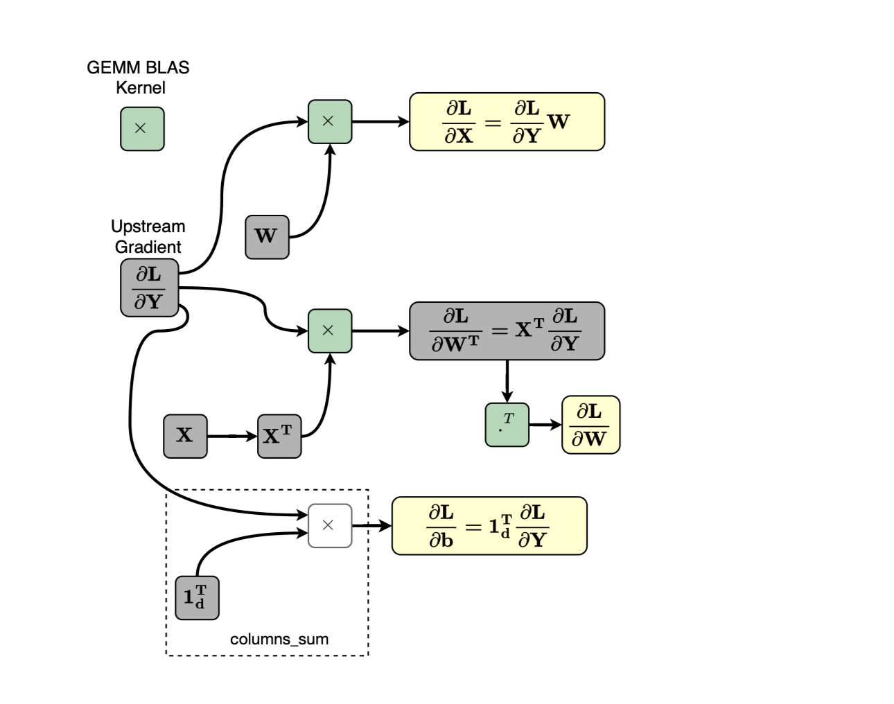
During the backward pass, the gradients with respect to \(\mathbf {W}\), \(\mathbf {b}\), and the input \(\mathbf {X}\) are computed. The gradients with respect to \(\mathbf {W}\) and \(\mathbf {X}\) are both evaluated using GEMM kernels (see figure below).
static variable_list AddmmBackward0_apply_functional(
  variable_list& grads,
....
{
...
  any_variable_defined(grads);
  if (needs_input_grad[/*mat1*/1]) {
    # dX
    auto grad_result = any_grad_defined ? (mm_mat1_backward(grad, mat2, mat1_sym_sizes, mat1_sym_strides, mat1_layout, alpha)) : Tensor();
    copy_range(grad_inputs, mat1_ix, grad_result);
  }
  if (needs_input_grad[/*mat2*/2]) {
    # dW^t
    auto grad_result = any_grad_defined ? (mm_mat2_backward(grad, mat1, mat2_sym_sizes, mat2_sym_strides, mat2_layout, alpha)) : Tensor();
    copy_range(grad_inputs, mat2_ix, grad_result);
  }
  if (needs_input_grad[/*self*/0]) {
    # db
    auto grad_result = any_grad_defined ? (maybe_multiply(grad, beta.conj())) : Tensor();
    copy_range(grad_inputs, self_ix, grad_result);
  }
  return grad_inputs;
}
Specifically, the gradient is first computed with respect to \(\mathbf {W}^{T}\), after which the TBackward node transposes it to obtain the gradient with respect to \(\mathbf {W}\) before it is accumulated by the AccumulateGrad node.
The sigmoid operator is one of the most widely used activation (non-linear) functions in deep learning, for example in binary classification (as we covered ealier). For a scalar input \(x \in \mathbb {R}\), the sigmoid function is defined as
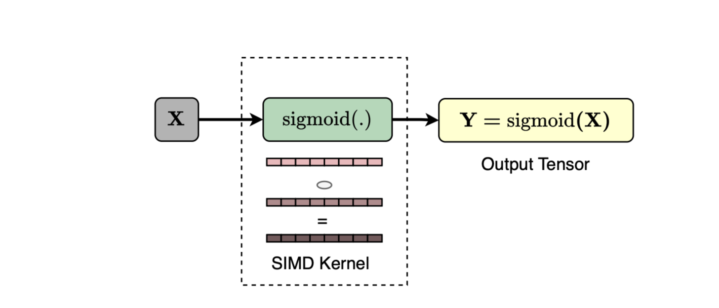
During the forward pass, the sigmoid function is applied element-wise to the input tensor \(\mathbf {X}\):
static void sigmoid_kernel(TensorIteratorBase& iter) {
...
 AT_DISPATCH_FLOATING_AND_COMPLEX_TYPES(dtype, "sigmoid_cpu", [&]() {
      cpu_kernel_vec(
          iter,
          [=](scalar_t a) -> scalar_t {
            return (static_cast<scalar_t>(1) / (static_cast<scalar_t>(1) + std::exp((-a))));
          },
          [=](Vectorized<scalar_t> a) {
            a = (Vectorized<scalar_t>(static_cast<scalar_t>(1)) + a.neg().exp()).reciprocal();
            return a;
          });
    });
  }
}
During the backward pass, the upstream gradient is multiplied element-wise by \(\mathbf {H}\) and \((1-\mathbf {H})\), where \(\mathbf {H}=\sigma (\mathbf {X})\):
where \(\odot \) denotes element-wise multiplication.
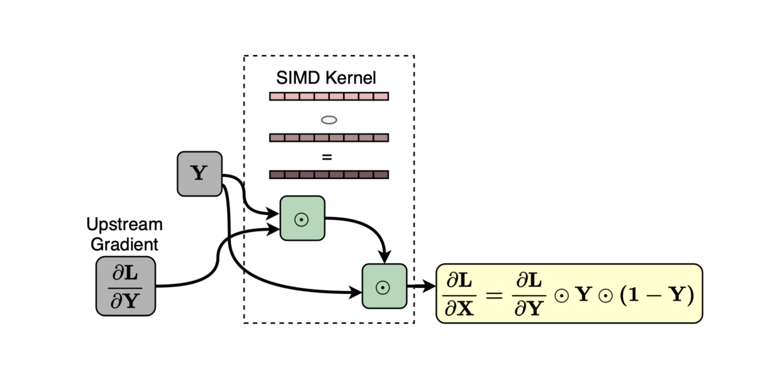
void sigmoid_backward_kernel(TensorIteratorBase& iter) {
...
    AT_DISPATCH_FLOATING_TYPES_AND(
        kHalf, iter.dtype(), "sigmoid_backward_cpu", [&]() {
          auto one_vec = Vectorized<scalar_t>((scalar_t)(1));
          cpu_kernel_vec(
              iter,
              [=](scalar_t a, scalar_t b) -> scalar_t {
                return a * (scalar_t(1) - b) * b;
              },
              [=](Vectorized<scalar_t> a, Vectorized<scalar_t> b) {
                return a * (one_vec - b) * b;
              });
        });
  }
}
Dropout consists of applying a randomly generated mask to the input tensor. Given a dropout probability \(p\), PyTorch samples an element-wise Bernoulli mask. During training, the output is scaled by a factor of \(\frac {1}{1-p}\) so that its expected value remains unchanged. This is illustrated below.
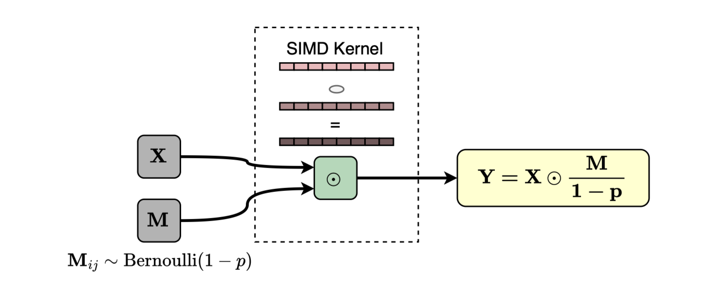
 template<bool feature_dropout, bool alpha_dropout, bool inplace, typename T>
Ctype<inplace> _dropout_impl(T& input, double p, bool train) {
 ...
  noise.bernoulli_(1 - p);
  ...
  if (alpha_dropout) {
    constexpr double alpha = 1.7580993408473766;
    double a = 1. / std::sqrt((alpha * alpha * p + 1) * (1 - p));
    b = noise.add(-1).mul_(alpha * a).add_(alpha * a * p);
    noise.mul_(a);
  } else {
    noise.div_(1 - p);
  }
  if (!alpha_dropout) {
    return multiply<inplace>(input, noise);
  } else {
    return multiply<inplace>(input, noise).add_(b);
  }
}
During backpropagation, the same scaled mask generated during the forward pass is reused. Specifically, the forward operation can be written as
where
For each element,
The gradient of \(\mathbf L\) with respect to \(\mathbf X_{ij}\) is obtained by contraction:
Since
all terms in the sum vanish except when \(k=i\) and \(l=j\). Therefore,
In tensor form,
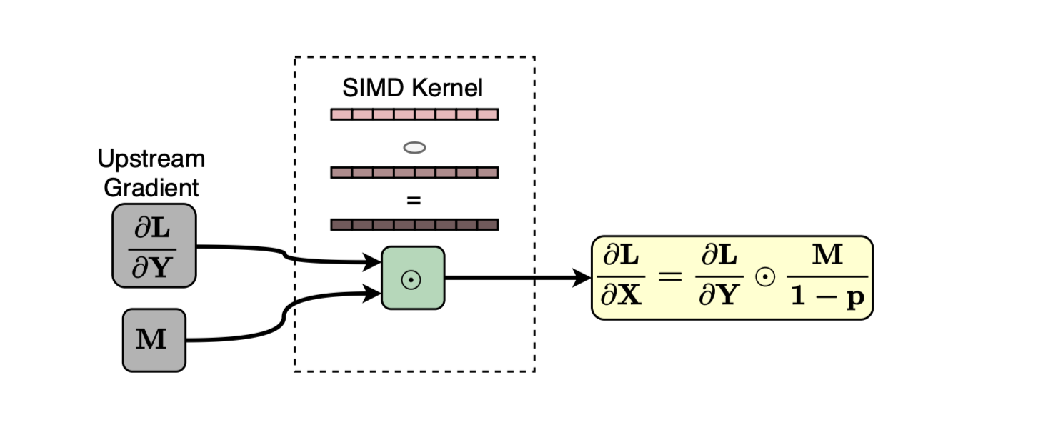
In PyTorch, this element-wise multiplication is represented in the autograd graph by a MulBackward0 node, which computes the gradient with respect to \(\mathbf {X}\) by multiplying the upstream gradient by the same scaled mask.
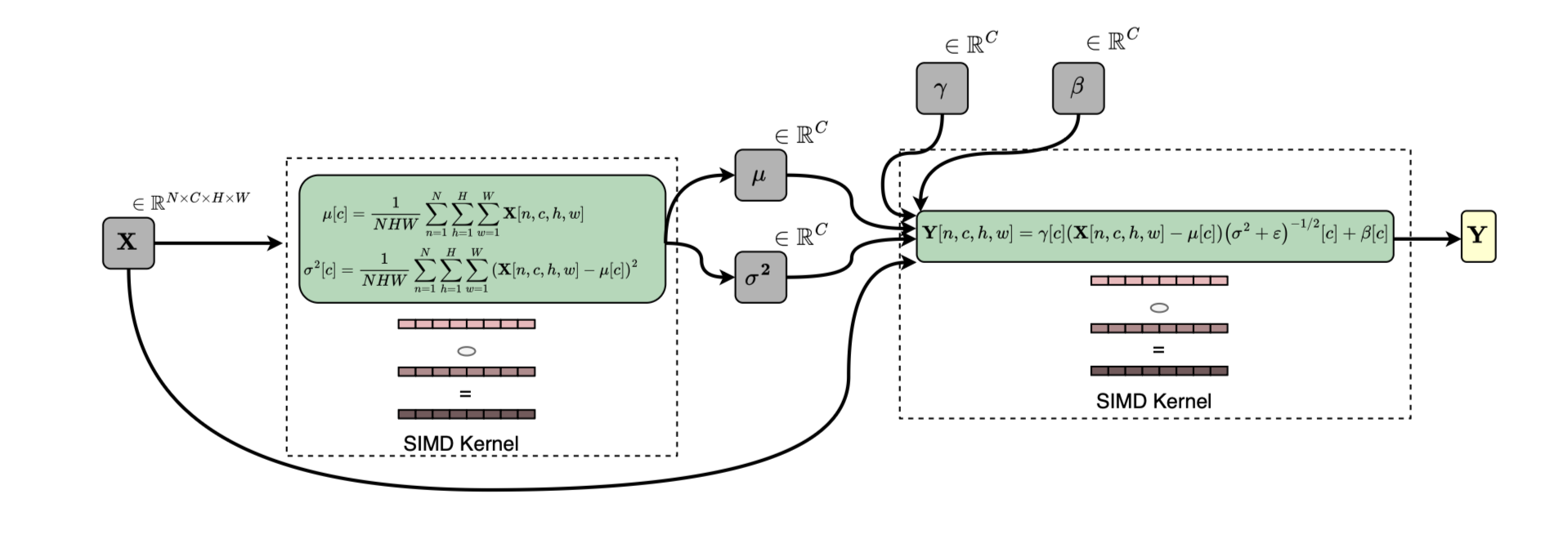
Given an input batch \(\mathbf {X} \in \mathbb {R}^{N \times C \times H \times W}\), Batch Normalization (BN) [?, ?] consists of normalizing the values independently for each feature channel:
Here, \(\boldsymbol {\mu }\) and \(\boldsymbol {\sigma }^2\) are vectors in \(\mathbb {R}^{C}\) containing the batch statistics computed independently for each feature channel, while \(\boldsymbol {\gamma }\) and \(\boldsymbol {\beta }\) are learnable vectors in \(\mathbb {R}^{C}\) used to scale and shift the normalized values. These parameters are learned during training through gradient-based optimization.
During the forward pass in training mode, PyTorch computes the mean and variance independently for each channel using the current mini-batch. First, for each channel, the mean over all samples and spatial locations is computed. Next, the variance is computed similarly for each channel. The data is then centered by subtracting the corresponding channel mean and normalized by dividing by the square root of the variance plus a small constant \(\varepsilon \) for numerical stability. Finally, a learnable scale and shift operation is applied.
PyTorch also maintains running estimates of the mean and variance during training. During inference, these running statistics are used instead of the statistics of the current batch. Batch Normalization helps mitigate vanishing and exploding gradients while stabilizing the training process. This is illustrated below.
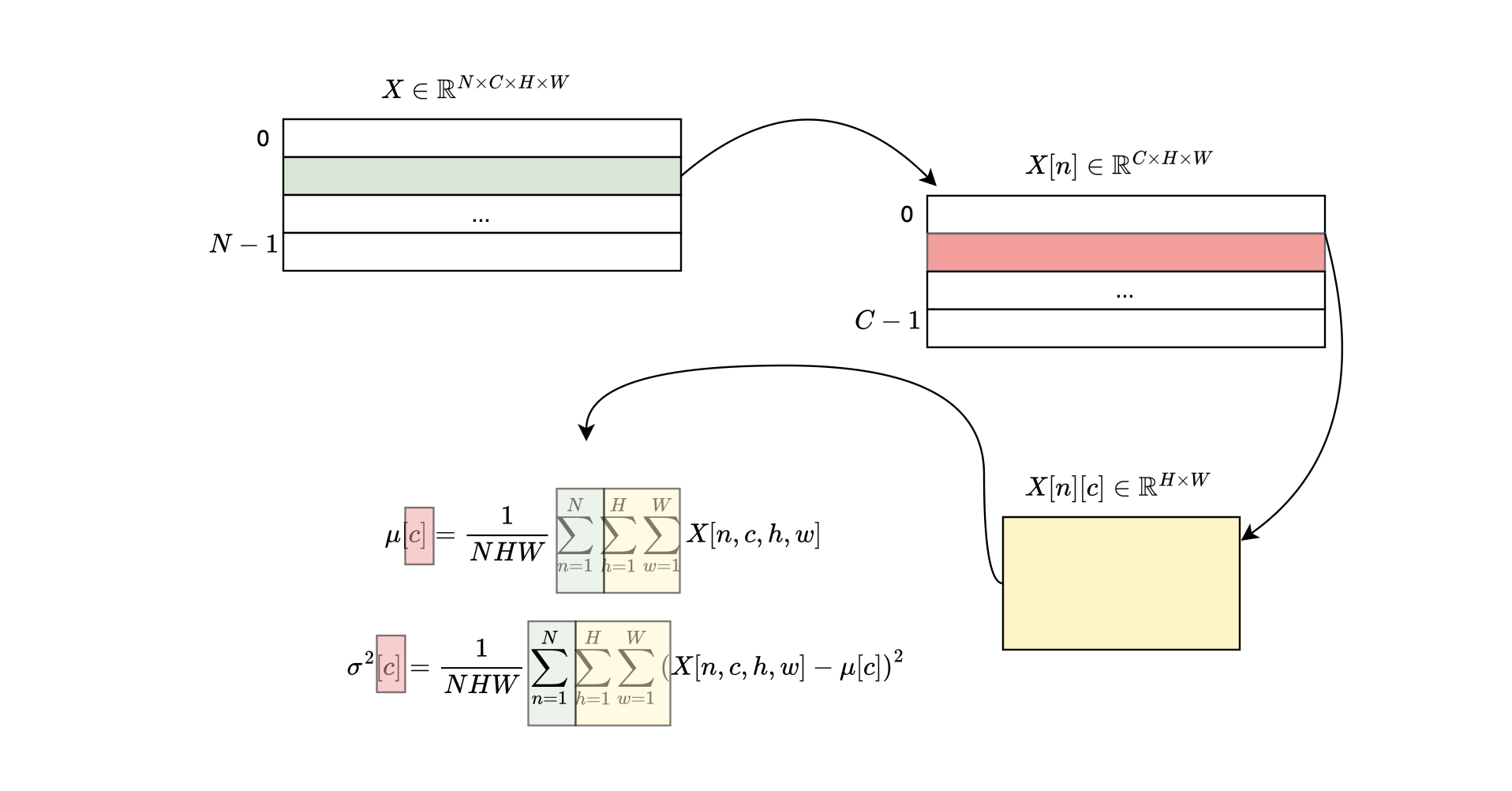
During the forward pass, PyTorch first computes the per-channel mean and variance, followed by an element-wise transformation to produce an output tensor of the same shape.
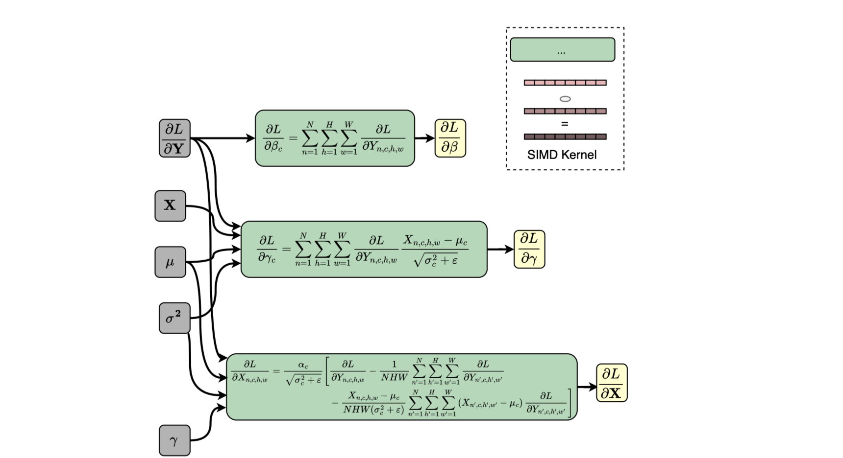
During the backward pass [?], the gradients with respect to the learnable scale and bias parameters are computed, both of which have simple closed-form expressions. The gradient with respect to the input, which is more involved, is then computed using the incoming gradient, assuming that the input tensor requires gradients.
Convolutional neural networks (CNNs) are one of the most successful deep learning techniques. They consist of convolving (or, more precisely, cross-correlating) an input image with a number of different kernels that are learned during training using SGD. Each local patch of the input image is contracted with a kernel of the same size.
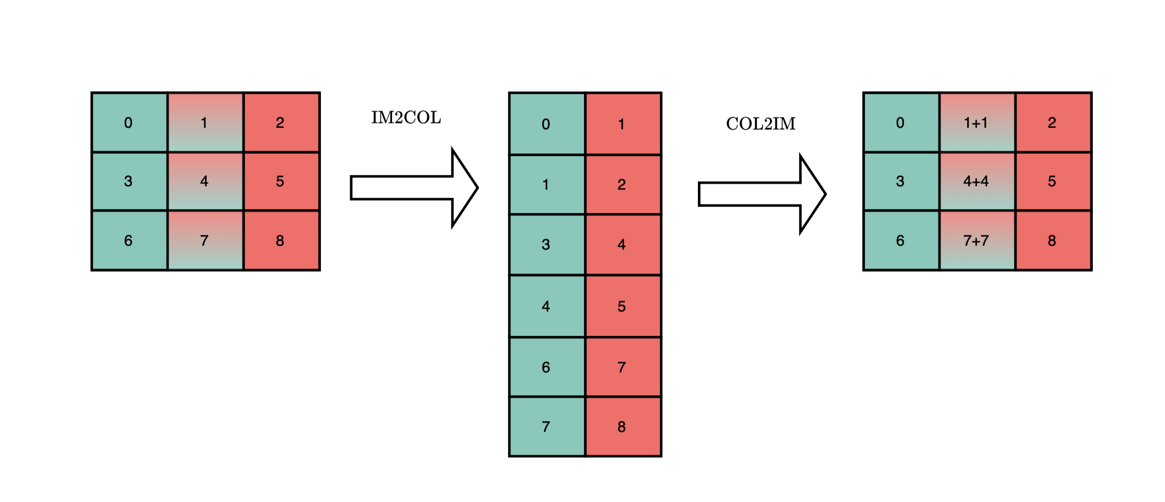
Instead of using a sliding-window approach, and to attain high performance, a common approach is to cast the convolution operation as a matrix multiplication (GEMM), which enables the use of highly optimized BLAS routines (e.g., Intel MKL, OpenBLAS). Each patch of the input image is unrolled into a column matrix using the im2col transformation.
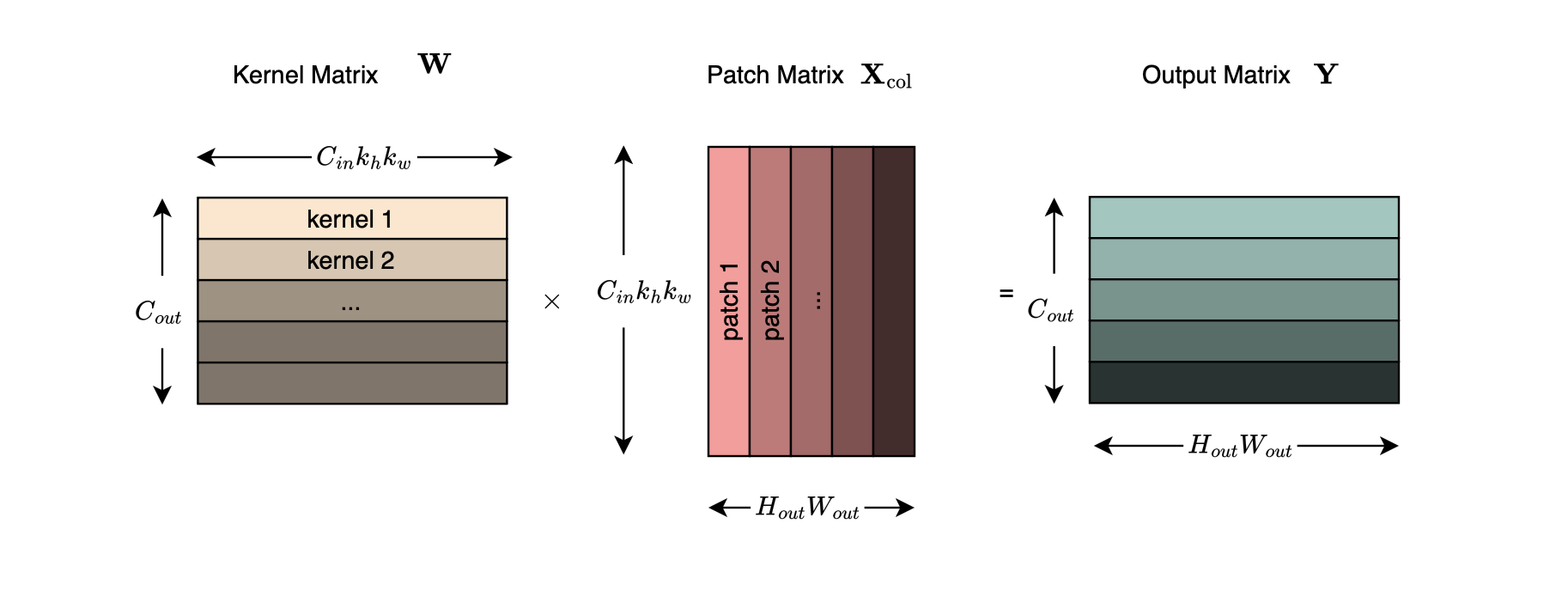
Assume that we have \(C_{\text {out}}\) kernels of size \(C_{\text {in}} \times k_h \times k_w\), where \(C_{\text {in}}\) is the number of input channels. These kernels, initially stored in the fourth-order tensor \(W\) of shape \((C_{\text {out}}, C_{\text {in}}, k_h, k_w)\), can be flattened and stacked into the weight matrix
Given an input image, the im2col transformation constructs a new patch matrix by unrolling patches from the input tensor into its columns:
In the simplest case, with unit stride and no padding, \(H_{\text {out}} = H_{\text {in}} - k_h + 1\) and \(W_{\text {out}} = W_{\text {in}} - k_w + 1\).The convolution mapping can be written as
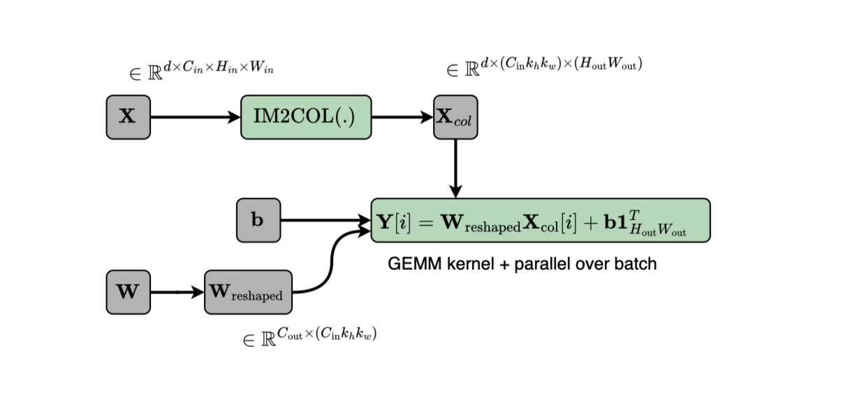
If we introduce a bias vector \(\mathbf {b} \in \mathbb {R}^{C_{\text {out}}}\) to shift each output channel, the operation becomes
During the forward pass, PyTorch iterates over the batch and performs one GEMM operation per sample.
Tensor& slow_conv2d_forward_out_cpu(
    const Tensor& self,
    const Tensor& weight_,
    IntArrayRef kernel_size, const std::optional<Tensor>& bias_opt,
    IntArrayRef stride,
    IntArrayRef padding,
    Tensor& output) {
  // See [Note: hacky wrapper removal for optional tensor]

  TORCH_CHECK(kernel_size.size() == 2, "2D kernel_size expected");
  TORCH_CHECK(stride.size() == 2, "2D stride expected");
  TORCH_CHECK(padding.size() == 2, "2D padding expected");

  c10::MaybeOwned<Tensor> bias_maybe_owned = at::borrow_from_optional_tensor(bias_opt);
  const Tensor& bias = *bias_maybe_owned;

  const int64_t kernel_height = kernel_size[0];
  const int64_t kernel_width = kernel_size[1];
  const int64_t pad_height = padding[0];
  const int64_t pad_width = padding[1];
  const int64_t stride_height = stride[0];
  const int64_t stride_width = stride[1];

  bool use_channels_last = thnn_conv_use_channels_last(self, weight_);
  auto memory_format = use_channels_last ? at::MemoryFormat::ChannelsLast : at::MemoryFormat::Contiguous;

  const Tensor weight_2d = view_weight_2d(weight_, memory_format);

  slow_conv2d_shape_check(
      self,
      Tensor(),
      weight_2d,
      bias,
      kernel_height,
      kernel_width,
      stride_height,
      stride_width,
      pad_height,
      pad_width,
      false);

  const Tensor input = self.contiguous(memory_format);
  const int64_t batch_size = input.size(0);
  const int64_t n_input_plane = input.size(1);
  const int64_t input_height = input.size(2);
  const int64_t input_width = input.size(3);
  const int64_t n_output_plane = weight_2d.size(0);
  const int64_t output_height = (input_height + 2 * pad_height - kernel_height) / stride_height + 1;
  const int64_t output_width = (input_width + 2 * pad_width - kernel_width) / stride_width + 1;

  Tensor finput = compute_columns2d(input, padding, stride, kernel_size, use_channels_last);
  output.resize_({batch_size, n_output_plane, output_height, output_width}, memory_format);
  if (bias.defined()) {
    output.copy_(bias.reshape({-1, 1, 1}));
  }
  TORCH_CHECK(output.is_contiguous(memory_format), "slow_conv2d output tensor must be contiguous");

  AT_DISPATCH_ALL_TYPES_AND2(kBFloat16, kHalf, input.scalar_type(), "slow_conv2d_cpu", [&]{
    auto input_a = input.accessor<const scalar_t, 4>();
    auto output_a = output.accessor<scalar_t, 4>();
    auto finput_a = finput.accessor<scalar_t, 3>();
    auto weight_2d_a = weight_2d.accessor<const scalar_t, 2>();

    at::parallel_for(0, batch_size, 0, [&](int64_t start, int64_t end) {
      for (const auto t : c10::irange(start, end)) {
        auto input_t = input_a[t];
        auto output_t = output_a[t];
        auto finput_t = finput_a[t];
        slow_conv2d_update_output_frame(
            input_t,
            output_t,
            weight_2d_a,
            bias.defined(),
            finput_t,
            kernel_height,
            kernel_width,
            stride_height,
            stride_width,
            pad_height,
            pad_width,
            n_input_plane,
            input_height,
            input_width,
            n_output_plane,
            output_height,
            output_width,
            use_channels_last);
      }
    });
  });

  return output;
}
This is illustrated below.
During the backward pass [?], considering the transformed upstream gradient
we need to compute the gradients with respect to the weight \(W\), bias \(\mathbf {b}\), and input \(\mathbf {X}\).
std::tuple<Tensor, Tensor, Tensor> slow_conv2d_backward_cpu(
    const Tensor& grad_output,
    const Tensor& self,
    const Tensor& weight,
    IntArrayRef kernel_size,
    IntArrayRef stride,
    IntArrayRef padding,
    std::array<bool, 3> output_mask) {
  Tensor grad_input;
  Tensor grad_weight;
  Tensor grad_bias;

  if (output_mask[0]) {
    grad_input = at::empty({0}, grad_output.options());
  }

  if (output_mask[1]) {
    grad_weight = at::empty({0}, grad_output.options());
  }

  if (output_mask[2]) {
    grad_bias = at::empty({0}, grad_output.options());
  }

  at::native::slow_conv2d_backward_out_cpu(
      grad_output,
      self,
      weight,
      kernel_size,
      stride,
      padding,
      grad_input,
      grad_weight,
      grad_bias);

  return std::make_tuple(
      std::move(grad_input), std::move(grad_weight), std::move(grad_bias));
}
The gradient with respect to the matricized kernel (or weight matrix) is similar to that of a linear layer, i.e.,
The gradient with respect to the kernel tensor is then obtained by reshaping the matrix,
which is again a fourth-order tensor.
For the bias vector, the gradient is given by
Now consider the gradient with respect to the input. We want to compute \(\frac {\partial L}{\partial \mathbf {X}}\); however, the input tensor is not used directly to compute the output. We therefore first compute
Given \(\frac {\partial L}{\partial \mathbf {X}_{\mathrm {col}}}\), the chain rule yields
where only the output positions \((k,l)\) to which \(\mathbf {X}_{i,j}\) contributes have a nonzero \(\frac {\partial (\mathbf {X}_{\mathrm {col}})_{k,l}} {\partial \mathbf {X}_{i,j}}\). It turns out that the gradient can be obtained by reversing the effect of im2col together with the required accumulation (col2im), i.e.,
Now assume we have \(d\) samples. The upstream gradient received by the autograd node is
where \(\left (\frac {\partial L}{\partial \mathbf {Y}}\right )_i\) refers to the upstream gradient for the \(i\)-th sample in the batch. To compute the gradient with respect to the matricized kernel, we accumulate the contribution from all samples,
due to the chain rule. As before, the reshape operator is then used to obtain \(\frac {\partial L}{\partial W}\).
Similarly, for the bias,
where \(\mathbf {1}_{H_{\text {out}}W_{\text {out}}}\) is a vector of ones. Observe that the matrix-vector multiplication above performs a contraction over the spatial dimension while the outer summation accumulates the result over the batch.
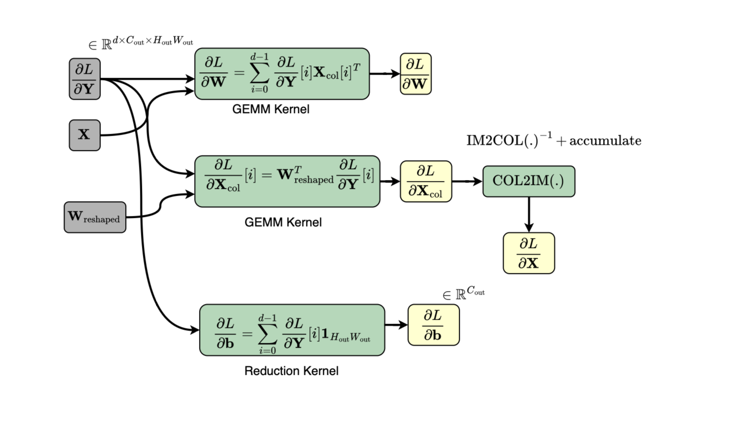
Finally, the gradient with respect to the input is computed independently for each sample,
template <typename scalar_t>
void slow_conv2d_backward_update_grad_input_frame(
    TensorAccessor<scalar_t, 3> grad_input,
    TensorAccessor<const scalar_t, 3> grad_output,
    TensorAccessor<const scalar_t, 2> weight,
    scalar_t *fgrad_input,
    int64_t kernel_height,
    int64_t kernel_width,
    int64_t stride_height,
    int64_t stride_width,
    int64_t pad_height,
    int64_t pad_width,
    bool is_channels_last) {
  // Compute fgrad_input = weight.T * grad_output.reshape({grad_output.shape(0), -1})
  // Note gemm expects fortran order, so all 3 matrices are transposed.
  // Swapping argument order cancels this, since C == AB <=> T(C) == T(B)T(A)
  if (is_channels_last) {
    const int64_t m = weight.size(1);
    const int64_t n = grad_output.size(1) * grad_output.size(2);
    const int64_t k = weight.size(0);

    const int64_t lda = m;
    const int64_t ldb = k;
    const int64_t ldc = m;

    at::native::cpublas::gemm(
        TransposeType::NoTranspose,
        TransposeType::NoTranspose,
        m, n, k,
        static_cast<scalar_t>(1),
        weight.data(), lda,
        grad_output.data(), ldb,
        static_cast<scalar_t>(0),
        fgrad_input, ldc);
  } else {
    const int64_t m = grad_output.size(1) * grad_output.size(2);
    const int64_t n = weight.size(1);
    const int64_t k = weight.size(0);

    const int64_t lda = m;
    const int64_t ldb = n;
    const int64_t ldc = m;

    at::native::cpublas::gemm(
        TransposeType::NoTranspose,
        TransposeType::Transpose,
        m, n, k,
        static_cast<scalar_t>(1),
        grad_output.data(), lda,
        weight.data(), ldb,
        static_cast<scalar_t>(0),
        fgrad_input, ldc);
  }

  unfolded2d_acc_stub(
      kCPU,
      c10::CppTypeToScalarType<scalar_t>::value,
      fgrad_input,
      grad_input.data(),
      kernel_height,
      kernel_width,
      stride_height,
      stride_width,
      pad_height,
      pad_width,
      grad_input.size(0),
      grad_input.size(1),
      grad_input.size(2),
      grad_output.size(1),
      grad_output.size(2),
      is_channels_last);
}
The MSE loss takes two tensors, the prediction \(\mathbf {Y}\) and the target \(\mathbf {T}\), as inputs, and computes the mean of the squared differences between their entries, i.e.,
where \(N\) denotes the total number of elements and \(\|\cdot \|_F\) denotes the Frobenius norm. For a matrix \(\mathbf {A}\in \mathbb {R}^{m\times n}\), the Frobenius norm is defined as
Consequently,
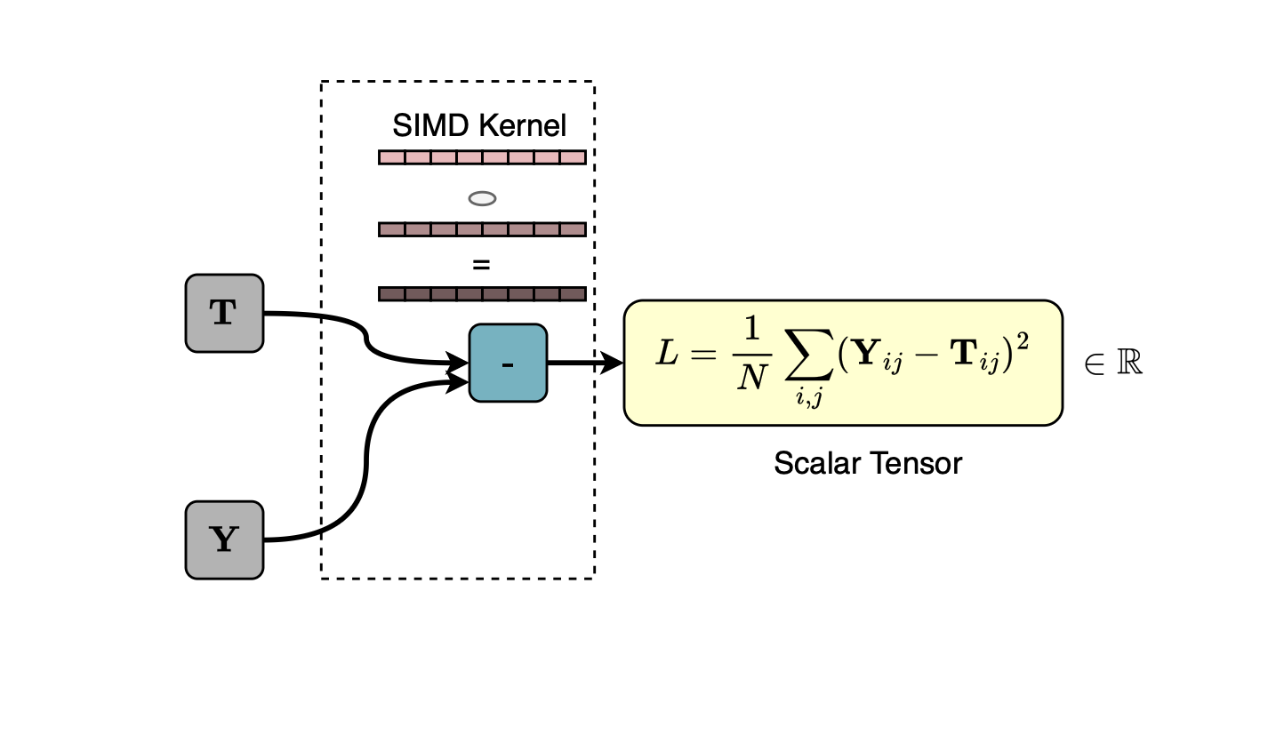
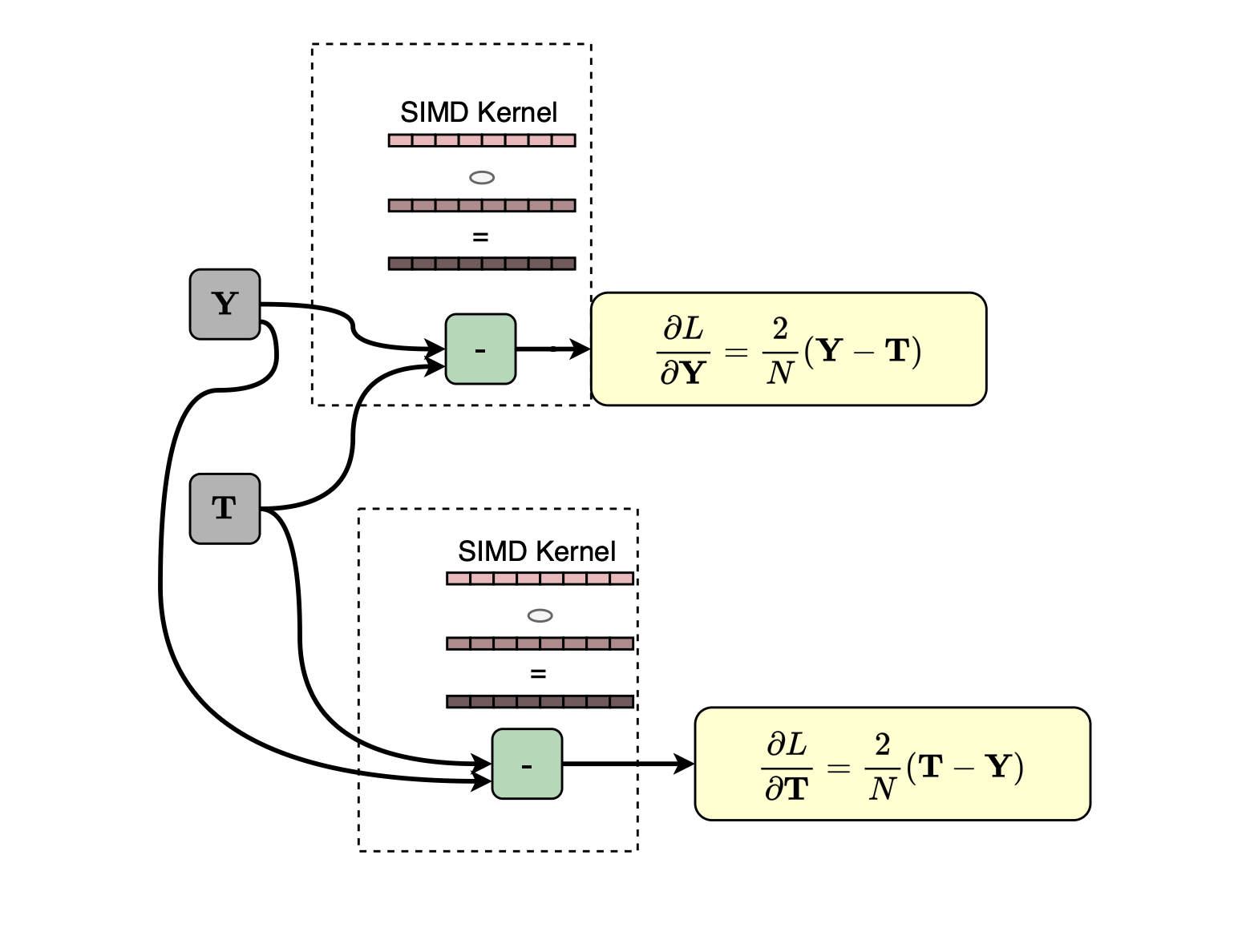
During backpropagation, the closed-form gradients are simpler than those of most other layers, as they reduce to element-wise subtraction and scaling:
and, if gradients with respect to the target are required,
as illustrated below.