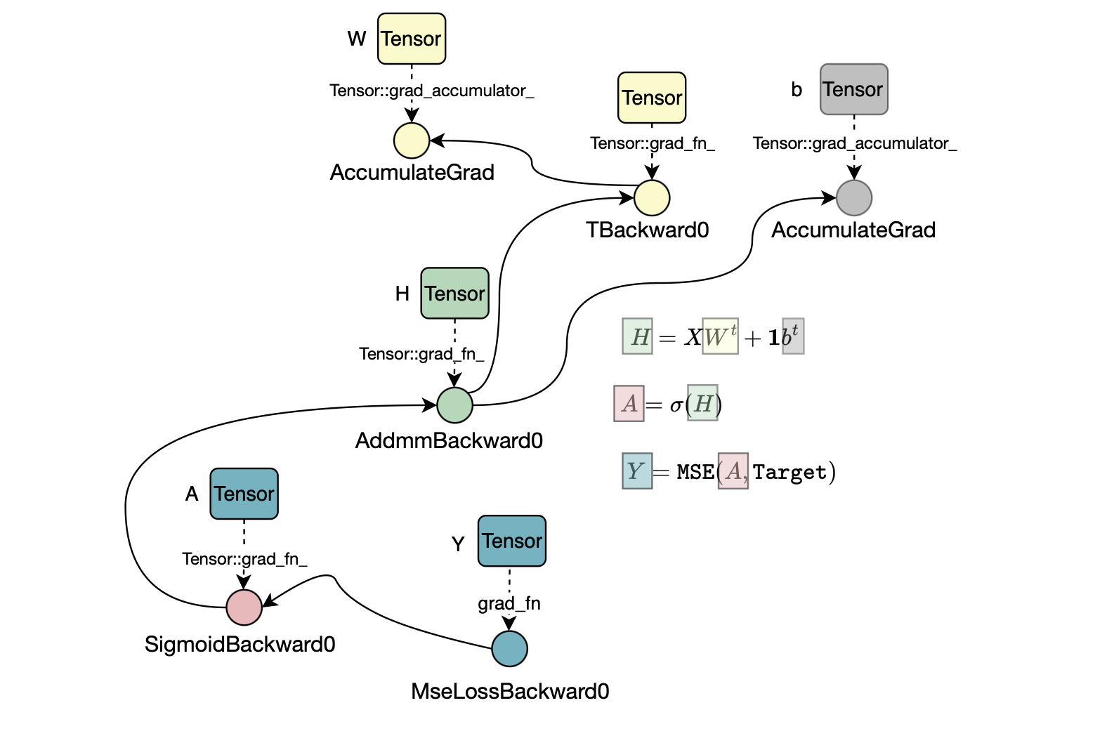
Deep learning models are trained using backpropagation, or more precisely, by repeatedly applying the chain rule of differentiation. Given a fixed neural network architecture, one can derive the gradient expressions and parameter update rules by hand and then implement them directly. However, every time the architecture changes, these derivations and their corresponding implementations must also be updated. This is precisely why frameworks such as PyTorch exist. During the forward pass, PyTorch records the executed differentiable operations to construct a computation graph. Each operation already has an associated backward implementation that computes its local derivatives. During the backward pass, the autograd engine traverses this graph in reverse, starting from the loss (or more generally, the tensor on which backward() is invoked), propagating gradients according to the chain rule until the leaf tensors are reached.
Deep learning models consist of a cascade of layers, where each layer may contain a set of learnable parameters, i.e., parameters that are updated during training. Backpropagation propagates gradients starting from the last layer, i.e., the one closest to the loss function, since this is where the gradient can first be computed and then propagated backward through the network.
As illustrated below, PyTorch constructs the computation graph during the forward pass. Specifically, each autograd kernel is first invoked through the dispatching mechanism before the actual backend implementation. The autograd kernel creates the corresponding autograd node, redispatches the operation to the target backend kernel, and receives the resulting tensor.
at::Tensor & addmm_(c10::DispatchKeySet ks, at::Tensor & self, const at::Tensor & mat1, const at::Tensor & mat2, const at::Scalar & beta, const at::Scalar & alpha) {
...

  c10::intrusive_ptr<AddmmBackward0> grad_fn;
  if (_any_requires_grad) {
   # Create autograd node
    grad_fn = c10::make_intrusive<AddmmBackward0>();
   # Collect edges !
    grad_fn->set_next_edges(collect_next_edges( self, mat1, mat2 ));
...
  # Redispatch
  {
    at::AutoDispatchBelowAutograd guard;
    at::redispatch::addmm_(ks & c10::after_autograd_keyset, self_, mat1_, mat2_, beta, alpha);
  }
The output tensor is then updated with the appropriate autograd metadata object used to hold the graph information, including connecting the output tensor to the autograd Node grad_fn which points to the graph node that will participate during the graph traversal to produce the local gradient given the upstream gradients. Next, the output tensor is served to the next layer. The subsequent layer inspects its input tensors, creates the corresponding backward edges, and thereby progressively constructs the entire computation graph (backward graph shown below is executed once the forward pass completes).
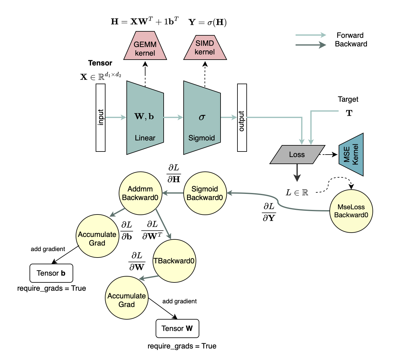
To reinforce our understanding so far, let us define a simple deep neural network, derive its computation graph by hand, and compare it with the computation graph generated by PyTorch. Consider an input \(\mathbf {X}\), and let
where \(\sigma (\cdot )\) denotes the sigmoid activation. The loss is defined as the mean squared error
The first quantity that can be computed immediately is the gradient of \(\mathbf {L}\) with respect to \(\mathbf {Y}\). Here, we assume that both \(\mathbf {Y}_{\text {target}}\) and \(\mathbf {X}\) do not require gradients. An example where \(\mathbf {X}\) does require gradients is during gradient-based adversarial attacks.
Once \(\frac {\partial \mathbf {L}}{\partial \mathbf {Y}}\) has been computed, we can derive the remaining gradients using the chain rule. For example,
where \(\frac {\partial \mathbf {Y}}{\partial \mathbf {W}_2^T}\) is itself a tensor rather than a simple matrix. Constructing this Jacobian explicitly would be prohibitively expensive. Instead, in PyTorch, as covered earlier, each backward function implements a closed-form expression, i.e., an analytical derivative, that directly computes the required gradient from the incoming gradient. The expression above should therefore be understood as the appropriate contraction between the incoming gradient and the Jacobian.
Similarly,
These dependencies define the first links of the computation graph. The node receiving \(\frac {\partial \mathbf {L}}{\partial \mathbf {Y}}\) computes both \(\frac {\partial \mathbf {L}}{\partial \mathbf {W}_2^T}\) and \(\frac {\partial \mathbf {L}}{\partial \mathbf {b}_2}\). The gradient with respect to \(\mathbf {b}_2\) is accumulated directly, whereas the gradient with respect to \(\mathbf {W}_2^T\) must be transposed to obtain the gradient with respect to \(\mathbf {W}_2\), requiring an additional node in the computation graph.
The same node also computes
which is propagated to the previous layer.
Next, we repeat the same procedure for the sigmoid layer. The sigmoid node receives \(\frac {\partial \mathbf {L}}{\partial \mathbf {H}_1}\) and computes
The resulting gradient \(\frac {\partial \mathbf {L}}{\partial \mathbf {A}_1}\) is then propagated backward to the preceding linear layer, where the same chain-rule computations are performed to obtain the gradients with respect to \(\mathbf {W}_1\), \(\mathbf {b}_1\), and, if necessary, the input \(\mathbf {X}\).
By representing all these dependencies as a graph, we obtain a computation graph containing ten nodes. Comparing with the one generated by PyTorch shows that they match exactly. This is, basically, how the autograd engine operates.
batch_size = 2
input_dim = 3
hidden_dim = 4
output_dim = 2
X = torch.randn(batch_size, input_dim)
Y_target = torch.randn(batch_size, output_dim)
linear1 = nn.Linear(input_dim, hidden_dim)
sigmoid = nn.Sigmoid()
linear2 = nn.Linear(hidden_dim, output_dim)
loss_fn = nn.MSELoss()
A1 = linear1(X)
H1 = sigmoid(A1)
Y = linear2(H1)
L = loss_fn(Y, Y_target)
L.backward()

print("AUTOGRAD GRAPH")
print("=" * 60)
print_graph(L.grad_fn)

#OUTPUT:

============================================================
AUTOGRAD GRAPH
============================================================
MseLossBackward0
    AddmmBackward0
        AccumulateGrad
        SigmoidBackward0
            AddmmBackward0
                AccumulateGrad
                TBackward0
                    AccumulateGrad
        TBackward0
            AccumulateGrad
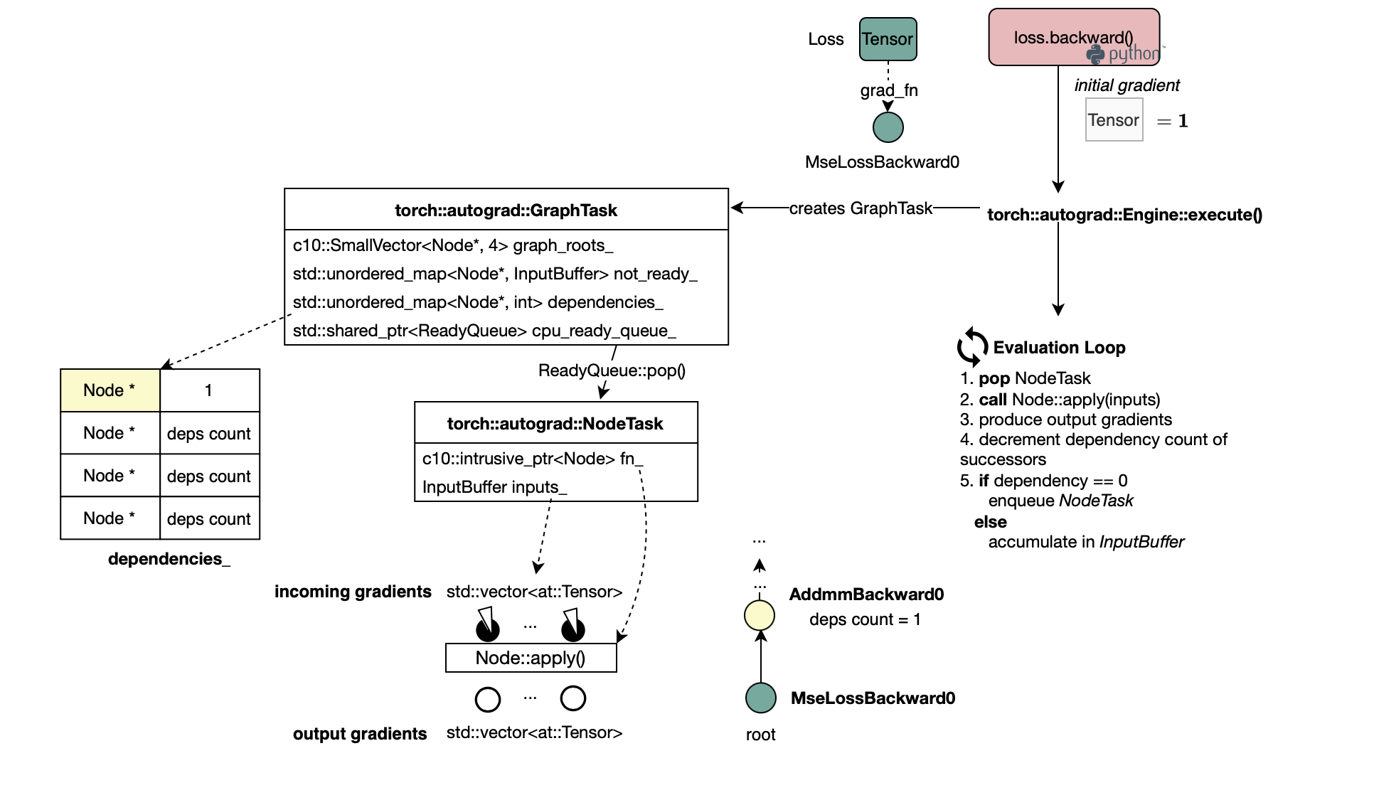
Given a computation graph, i.e., a set of root nodes (from now on assuming a single root node for simplicity), the autograd engine executes the graph starting from the root node and then successively invokes the nodes that are ready for execution. Specifically, it maintains a dependency count for each node to determine whether all of its incoming gradients are available. The root node is executed first, and its output gradients are propagated along the outgoing edges. For each successor node, the dependency count is decremented; once it reaches zero, a dedicated NodeTask is created and enqueued for execution. This process continues until all nodes in the computation graph have been evaluated, at which point the autograd engine returns. This is illustrated below.
Once the backward pass has completed, the underyling optimizer is invoked to update the parameters.
d = 4
n = 3
m = 2

X = torch.randn(d, n)
W = torch.randn(m, n, requires_grad=True)
b = torch.randn(m, requires_grad=True)
T = torch.randn(d, m)
H = torch.addmm(b, X, W.t())
A = torch.sigmoid(H)
error = F.mse_loss(A, T, reduction="mean")

print("W.grad_fn =", W.grad_fn)
print("b.grad_fn =", b.grad_fn)
print("H.grad_fn =", H.grad_fn)
print("A.grad_fn =", A.grad_fn)
print("error.grad_fn =", error.grad_fn)


print_autograd_graph(error.grad_fn)

#OUTPUT

MseLossBackward0
    SigmoidBackward0
        AddmmBackward0
            AccumulateGrad  <-- b
            TBackward0
                AccumulateGrad  <-- W